
ENGG-401 · Lesson 12 of 12 · 30 min
Risk, sensitivity and decision analysis, and capstone
Every number in an engineering economic analysis is an estimate. First costs may overrun, savings may fall short, lives may be shorter or longer than expected, and interest rates, prices and regulations may change. A present worth of $21,460 is not a fact; it is the result of a particular set of assumptions. Good analysis shows decision-makers how robust the conclusion is: which estimates matter most, how much they would have to change to reverse the decision, and what the range of possible outcomes looks like. This final lesson covers sources of uncertainty, sensitivity analysis and tornado diagrams, break-even analysis, scenario analysis, expected values and probability, decision trees and the value of information, Monte Carlo simulation, real options, communicating uncertainty, and the course capstone.
Sources of uncertainty
Uncertainty arises from many sources: inaccurate estimates of quantities and prices; market demand and competition; technological performance and reliability; construction risks such as ground conditions and weather; inflation, interest and exchange rates; regulation and policy, including taxes and environmental rules; and project duration and asset life. Some risks can be reduced by better information, such as geotechnical investigations or pilot tests; some can be transferred, through insurance, contracts or hedging; and some must simply be accepted and priced. Distinguishing risk, where probabilities can be estimated, from deep uncertainty, where they cannot, helps choose appropriate methods.
Sensitivity analysis
Sensitivity analysis changes one input at a time, holding the others at their base values, and observes the effect on the measure of worth. It identifies the inputs to which the decision is most sensitive, so that estimation effort and risk management can focus on them.
Worked problem
Sensitivity of the inspection system
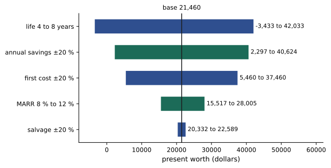
For the inspection system (base PW $21,460 at 10 %), find the PW when each input changes by ±20 %, and when life is 4 or 8 years and the MARR is 8 % or 12 %.
Show solution
- Annual savings ±20 % ($17,600 to $26,400): PW from $2,300 to $40,620.
- First cost ±20 % ($64,000 to $96,000): PW from $37,460 to $5,460.
- Salvage ±20 %: PW from $20,330 to $22,590.
- Life 4 or 8 years: PW from −$3,430 to $42,030; MARR 8 % or 12 %: PW from $28,010 to $15,520.
Answer: The decision is most sensitive to annual savings and life, moderately to first cost and MARR, and hardly at all to salvage value.
The results are commonly shown in a spider plot, with PW plotted against the percentage change in each input, steeper lines indicating greater sensitivity, or in a tornado diagram, horizontal bars showing the PW range for each input, sorted from widest to narrowest.
Break-even analysis
Break-even analysis finds the value of an input at which the decision changes, typically where PW equals zero or where two alternatives are equally attractive. It answers the question decision-makers often care about most: how wrong could this estimate be before we regret the decision? For the inspection system, the break-even annual savings satisfy \(-80{,}000 + A\,(P/A, 10\,\%, 6) + 10{,}000\,(P/F, 10\,\%, 6) = 0\), giving \(A = 17{,}073\): savings could fall by 22 % before the investment ceases to earn the MARR. The break-even life, with the salvage value unchanged, is about 4.3 years. Break-even analysis is also used for make-or-buy decisions, for choosing between alternatives with different fixed and variable costs, and for finding the production volume at which a business covers its costs.
Worked problem
Make or buy
A plant can buy a component for $14 each or make it with equipment that has an equivalent annual cost of $90,000 plus $8 per unit. At what annual volume is making cheaper?
Show solution
- Cost to buy: \(14Q\); cost to make: \(90{,}000 + 8Q\).
- Break-even: \(14Q = 90{,}000 + 8Q\), so \(Q = 15{,}000\) units.
- Above 15,000 units a year, making is cheaper; below, buying is.
Answer: Make the component if annual demand reliably exceeds 15,000 units.
Scenario analysis
Sensitivity analysis changes one input at a time, but in reality inputs often move together: a recession may reduce demand, prices and utilization simultaneously. Scenario analysis defines consistent sets of assumptions, such as optimistic, most likely and pessimistic cases, or scenarios tied to specific events such as a carbon price, a new competitor or a change in regulation, and computes the measure of worth for each. Scenarios help decision-makers understand the range of outcomes and plan responses, though they do not by themselves indicate how likely each outcome is.
Expected value and risk
When probabilities can be assigned to outcomes, the expected value of a measure of worth is the probability-weighted average of its possible values, \(E[PW] = \sum p_k\,PW_k\). A risk-neutral decision-maker chooses the alternative with the highest expected present worth. But expected value alone ignores the spread of outcomes: two projects with the same expected value may differ greatly in their chance of loss. The variance or standard deviation of PW, the probability of a negative PW, and the worst plausible outcome are all useful additional measures. Organizations are often risk-averse, particularly when a loss could threaten the business, and may prefer a project with a slightly lower expected value and much less risk.
Decision trees
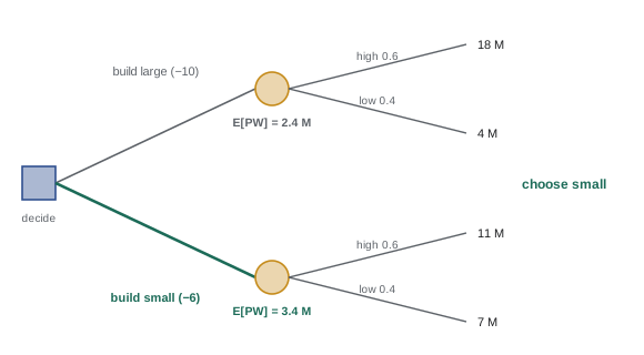
Decision trees structure decisions made in sequence under uncertainty. Square nodes represent decisions, circular nodes represent chance events with probabilities, and branches end in outcomes valued by their present worth. The tree is solved by rolling back from the end: at each chance node, compute the expected value; at each decision node, choose the branch with the highest expected value. Decision trees are valuable when a decision can be staged, when information will arrive over time, and when the option to change course later has value.
Worked problem
Large plant or small plant
A company can build a large plant costing $10 million or a small plant costing $6 million. Demand will be high with probability 0.6 or low with probability 0.4. The present worth of operating revenues net of operating costs is $18 million (high) or $4 million (low) for the large plant, and $11 million (high, including the option to expand) or $7 million (low) for the small plant. Which should be built, and what is the value of perfect information about demand?
Show solution
- Large: \(E[PW] = 0.6 \times 18 + 0.4 \times 4 - 10 = 2.4\) million.
- Small: \(E[PW] = 0.6 \times 11 + 0.4 \times 7 - 6 = 3.4\) million; build small.
- With perfect information: choose large if demand is high (PW 8) and small if low (PW 1); expected value \(0.6 \times 8 + 0.4 \times 1 = 5.2\) million.
- Expected value of perfect information: \(5.2 - 3.4 = 1.8\) million.
Answer: Build the small plant (expected PW $3.4 million); a market study costing up to $1.8 million could in principle be worthwhile, although real studies give imperfect information worth less.
Monte Carlo simulation
When many inputs are uncertain at once, Monte Carlo simulation provides a full probability distribution of outcomes. Each uncertain input is described by a probability distribution, such as triangular, uniform, normal or based on historical data; the model draws a random value for each input, computes the measure of worth, and repeats thousands of times. The results show the expected value, the spread, the probability of a negative present worth and percentiles such as the 10th and 90th (often called P10 and P90). Correlations between inputs, such as demand and price, should be modelled where they exist. Spreadsheet add-ins and programming languages make Monte Carlo simulation accessible, and it is standard practice in oil and gas, mining, major projects and cost estimating.
Worked problem
Simulating the inspection system
Suppose annual savings follow a triangular distribution from $15,000 to $28,000 with a mode of $22,000, life is equally likely to be 4, 5, 6, 7 or 8 years, salvage is uniform between $5,000 and $15,000, and first cost is triangular from $75,000 to $95,000 with a mode of $80,000. What does a simulation of 100,000 trials at 10 % show?
Show solution
- Expected PW: about $15,600, lower than the deterministic $21,460 because the first cost distribution is skewed upward and savings slightly downward.
- Probability of a negative PW: about 25 %.
- Fifth and ninety-fifth percentiles: about −$15,700 and +$49,900.
Answer: The investment is attractive on average, but there is roughly a one-in-four chance it will not earn the MARR, information the deterministic analysis hides.
Real options
Traditional present worth analysis assumes a fixed plan, but managers can adapt: they can delay an investment until uncertainty resolves, expand if demand is high, switch fuels or products, or abandon a failing project. These flexibilities, called real options, have value that a static analysis ignores. The small plant in the decision tree is worth more partly because of its option to expand. Designing flexibility into engineering systems, such as modular plants, reserved space for future expansion, or equipment that can run on multiple fuels, can be worth more than optimizing for a single forecast. Real options analysis uses decision trees, simulation or option pricing methods adapted from finance.
Communicating uncertainty
Decision-makers need to understand both the expected outcome and the risks. Good practice includes presenting the base case with its key assumptions; showing a tornado diagram and break-even values; presenting scenarios or probability distributions where appropriate; stating which risks can be reduced, transferred or must be accepted; and recommending risk management actions. Avoid false precision: reporting a present worth of $21,460.47 implies accuracy the estimates do not have. Honest communication of uncertainty is part of an engineer's professional responsibility and builds trust with clients, employers and the public.
Capstone: an engineering economic study
The capstone asks you to prepare a complete engineering economic study of a real or realistic engineering decision, such as an energy retrofit, equipment replacement, process improvement, infrastructure upgrade, renewable energy installation or make-or-buy decision. Your report should include:
- A problem statement with the objective, constraints and feasible alternatives, including the do-nothing or base case.
- Cash flow estimates for each alternative with sources, accuracy and assumptions, and cash flow diagrams.
- A justified MARR or social discount rate, stated as real or nominal.
- Analysis by present worth or annual worth, with incremental rate of return or benefit-cost analysis where appropriate.
- An after-tax analysis using the tax rules of your country (CCA or MACRS and current incentives), and treatment of inflation.
- A replacement or economic life analysis if relevant.
- Sensitivity, break-even and either scenario, decision tree or Monte Carlo analysis.
- Discussion of non-monetary factors, risks and professional responsibilities, and a clear recommendation.
Present it as a professional report of about 3,000 words with supporting spreadsheets, suitable for a manager or client.
Risk-adjusted discount rates and certainty equivalents
Two common ways to account for risk in present worth are risk-adjusted discount rates and certainty equivalents. A risk-adjusted discount rate raises the MARR for riskier projects, which reduces the present worth of distant cash flows more heavily; it is simple and widely used but implicitly assumes that risk grows steadily with time. The certainty equivalent approach reduces uncertain cash flows to the amounts a decision-maker would accept with certainty, then discounts them at a risk-free rate; it is more transparent about the treatment of risk but harder to apply. In practice, firms often combine risk classes for MARR with explicit sensitivity and probabilistic analysis.
Common mistakes
MistakePresenting a single PW as certain.
InsteadShow sensitivity, break-even and ranges.
MistakeVarying correlated inputs independently.
InsteadUse scenarios or correlated simulation.
MistakeChoosing by expected value alone when losses are severe.
InsteadConsider spread and probability of loss.
MistakeIgnoring the value of flexibility.
InsteadUse decision trees or real options for staged decisions.
MistakeReporting results with false precision.
InsteadRound to match estimate accuracy.
Summary and key terms
- All economic analyses rest on uncertain estimates.
- Sensitivity analysis and tornado diagrams identify the most important inputs.
- Break-even analysis shows how far an estimate can move before the decision changes.
- Scenarios vary inputs together; expected value and spread describe risk.
- Decision trees handle sequential decisions and value information.
- Monte Carlo simulation produces full distributions of outcomes.
- Real options value flexibility; communicate uncertainty honestly.
- Sensitivity analysis
- Changing one input at a time to see its effect.
- Tornado diagram
- Bars showing output ranges for each input.
- Spider plot
- Lines of output versus percentage change in inputs.
- Break-even value
- Input value at which the decision changes.
- Scenario analysis
- Evaluating consistent sets of assumptions.
- Expected value
- Probability-weighted average outcome.
- Decision tree
- Diagram of sequential decisions and chance events.
- EVPI
- Expected value of perfect information.
- Monte Carlo simulation
- Repeated random sampling of uncertain inputs.
- Real option
- Value of managerial flexibility.
Practice problems
Work each problem on paper first, then reveal the answer to check.
What does sensitivity analysis vary?
Show answer
One input at a time.
Which input most affects the inspection system?
Show answer
Annual savings and life.
Break-even annual savings for the system?
Show answer
About $17,073.
Break-even volume for fixed $50,000, price $20, variable $15?
Show answer
10,000 units.
Why use scenarios?
Show answer
Inputs often change together.
Expected PW of 0.3 × 50 and 0.7 × (−10) thousand?
Show answer
$8,000.
How is a decision tree solved?
Show answer
Roll back: expected values at chance nodes, best choice at decision nodes.
What is EVPI?
Show answer
Expected value with perfect information minus best expected value without it.
Name two outputs of Monte Carlo simulation.
Show answer
Expected value, probability of loss, percentiles.
Give an example of a real option.
Show answer
Delay, expand, switch or abandon.
Lesson quiz · 5 questions
Score 60% or more to complete this lesson.
Create a free account to save your progress, take quizzes and earn a certificate.