
ELE-390 · Lesson 9 of 12 · 25 min
Frequency response: Bode and Nyquist plots
The root locus works with pole and zero locations, which must come from a model. The frequency response works with gain and phase at each frequency, which can also come from a measurement. That is the great practical strength of frequency-domain methods: an engineer can drive a real loop with sinusoids, or with a swept-sine or noise signal, record the response, and judge its stability and robustness without ever writing down a transfer function. This lesson reviews Bode plots from ELE-250, applies them to the PT-1 loop, and introduces the Nyquist stability criterion and the two stability margins that lesson 10 designs with.
Sinusoidal steady state
When a stable linear system is driven by a sinusoid A sin ωt, its output, after the transients die away, is a sinusoid at the same frequency, A|G(jω)| sin(ωt + ∠G(jω)). The frequency response G(jω) is the transfer function evaluated on the imaginary axis. Its magnitude is the gain at that frequency and its angle is the phase shift. For a loop, the most useful frequency response is that of the loop gain L(jω) = C(jω)G(jω), because the closed loop's behaviour, and its stability, can be read from it.
Leo measures it on the PT-1 bench by breaking the loop in software: the controller is replaced by a sinusoidal voltage source of a few volts, the encoder is logged, and the camera's angle is compared with the drive in amplitude and phase at 30 frequencies from 0.3 to 300 rad/s. Because the plant contains an integrator, the camera would drift away in open loop, so he keeps a weak proportional loop closed around it, a few volts per radian, and computes the open-loop response from the closed-loop data. That is standard practice for unstable or marginally stable plants.
Bode plots
A Bode plot shows the magnitude in decibels, 20 log₁₀|G|, and the phase in degrees, both against frequency on a logarithmic axis. Logarithms turn products into sums, so the Bode plot of a product of factors is the sum of the factors' plots, and each standard factor has a simple straight-line approximation.
| Factor | Magnitude asymptote | Phase |
|---|---|---|
| Constant K | Flat at 20 log K | 0° (or −180° if K < 0) |
| Integrator 1/s | −20 dB/decade, 0 dB at ω = 1 | −90° |
| Real pole 1/(s/a + 1) | 0 dB below a, −20 dB/decade above; −3 dB at a | 0° to −90°, −45° at a |
| Real zero s/a + 1 | 0 dB below a, +20 dB/decade above | 0° to +90°, +45° at a |
| Complex pole pair ω_n²/(s² + 2ζω_ns + ω_n²) | 0 dB below ω_n, −40 dB/decade above; peak near ω_n if ζ < 0.7 | 0° to −180°, −90° at ω_n, steep when ζ is small |
| Delay e^{−θs} | 0 dB at all frequencies | −ωθ radians, without limit |
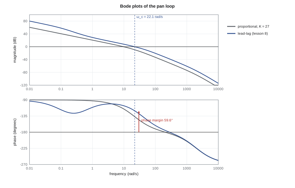
The pan plant G(s) = 16 667/(s(s + 21.2)(s + 1979)) has three factors besides its gain: the integrator, the mechanical pole at 21.2 rad/s and the electrical pole at 1979 rad/s. Its magnitude falls at −20 dB/decade from low frequency, steepens to −40 dB/decade above 21.2 rad/s and to −60 dB/decade above 1979 rad/s. Its phase starts at −90°, passes −135° at 21.2 rad/s and approaches −270° far above 1979 rad/s. Each compensator from lesson 8 adds its own factors: the lead adds a zero at 21.2, cancelling the mechanical pole's contribution, and a pole at 40; the lag adds a zero at 0.5 and a pole at 0.125.
Stability margins
A loop with unity negative feedback is at the edge of stability when L(jω) = −1 at some frequency: magnitude one, phase −180°. Two numbers measure how far the loop is from that condition. The gain margin is how much the loop gain could rise before the loop became unstable: at the phase crossover frequency ω₁₈₀, where the phase is −180°, it is 1/|L(jω₁₈₀)|, usually quoted in decibels. The phase margin is how much additional phase lag the loop could tolerate: at the gain crossover frequency ω_c, where |L| = 1 (0 dB), it is 180° plus the phase there.
Typical targets are a gain margin of 6 to 12 dB and a phase margin of 45° to 65°. The phase margin is also closely tied to the damping of the dominant closed-loop poles: for a second-order loop, ζ ≈ PM/100 for phase margins up to about 60°, so 60° of margin gives ζ ≈ 0.6 and about 10 % overshoot. The crossover frequency ω_c is close to the closed-loop bandwidth, and a common rule is that the settling time is roughly 8/ω_c to 10/ω_c for well-damped loops. These rules let a designer translate the time-domain specifications of lesson 4 into frequency-domain ones.
import math, cmath
G = lambda s: 16667 / (s * (s + 21.2) * (s + 1979))          # volts to camera radians
designs = {
    "P, K = 27":  lambda s: 27.0,
    "lead":       lambda s: 133.0 * (s + 21.2) / (s + 40),
    "lead-lag":   lambda s: 120.0 * (s + 21.2) * (s + 0.5) / ((s + 40) * (s + 0.125)),
}
def db(x): return 20 * math.log10(abs(x))
def phase(x): return math.degrees(cmath.phase(x))
def unwrap_phase(L, w):  # continuous phase from low frequency upward
    ws = [10 ** (k / 400) for k in range(-1200, int(400 * math.log10(w)) + 1)]
    ph, prev = 0.0, None
    for wk in ws:
        p = cmath.phase(L(1j * wk))
        if prev is None: ph = p
        else:
            d = p - prev
            while d > math.pi: d -= 2 * math.pi
            while d < -math.pi: d += 2 * math.pi
            ph += d
        prev = p
    return math.degrees(ph)
def crossing(f, lo, hi):
    for _ in range(80):
        mid = math.sqrt(lo * hi)
        lo, hi = (mid, hi) if f(mid) > 0 else (lo, mid)
    return math.sqrt(lo * hi)
print("Bode points of the lead-lag loop:")
Lll = lambda s: designs["lead-lag"](s) * G(s)
for w in (0.1, 0.5, 1, 5, 10, 30, 60, 100, 200, 1000, 2000):
    print(f"  w = {w:6.1f} rad/s: |L| = {db(Lll(1j*w)):6.1f} dB, phase {unwrap_phase(Lll, w):7.1f} deg")
print("margins:")
for name, C in designs.items():
    L = lambda s, C=C: C(s) * G(s)
    wc = crossing(lambda w: abs(L(1j * w)) - 1, 0.1, 5000)            # gain crossover
    pm = 180 + unwrap_phase(L, wc)
    w180 = crossing(lambda w: unwrap_phase(L, w) + 180, 1, 5000)        # phase crossover
    gm = -db(L(1j * w180))
    print(f"  {name:10s} crossover {wc:6.1f} rad/s, PM {pm:5.1f} deg; phase crossover {w180:6.1f} rad/s, GM {gm:5.1f} dB")
# Nyquist test of proportional control beyond the Routh limit: count encirclements of -1
def encirclements(L, w_lo=1e-3, w_hi=1e5, n=200000):
    # the contour avoids the pole at the origin with a small right-hand detour; count net winding of 1 + L
    pts = [1j * 10 ** (math.log10(w_lo) + (math.log10(w_hi) - math.log10(w_lo)) * k / n) for k in range(n + 1)]
    path = [complex(-z.real, -z.imag) for z in reversed(pts)] + pts   # -j infinity ... +j infinity
    eps = w_lo
    arc = [eps * cmath.exp(1j * th) for th in [(-math.pi / 2 + math.pi * k / 200) for k in range(201)]]
    contour = path[:len(pts)] + arc + path[len(pts):]
    total = 0.0; prev = None
    for s in contour:
        v = 1 + L(s); a = cmath.phase(v)
        if prev is not None:
            d = a - prev
            while d > math.pi: d -= 2 * math.pi
            while d < -math.pi: d += 2 * math.pi
            total += d
        prev = a
    return -round(total / (2 * math.pi))   # clockwise count (the large arc maps to a point and adds nothing)
for K in (1000.0, 6000.0):
    print(f"P control K = {K:.0f}: clockwise encirclements of -1 = {encirclements(lambda s: K * G(s))}")
# the cabinet with 90 s delay is handled exactly: phase -atan(3000 w) - 90 w
for Kc in (150.0, 300.0):
    L = lambda s: Kc * 0.1 * cmath.exp(-90 * s) / (3000 * s + 1)
    wc = crossing(lambda w: abs(L(1j * w)) - 1, 1e-6, 1)
    pm = 180 - math.degrees(math.atan(3000 * wc)) - math.degrees(90 * wc)
print(f"cabinet Kc = {Kc:.0f} W/K: crossover {wc*1000:.2f} mrad/s, PM {pm:.1f} deg, GM {20*math.log10(530/Kc):.1f} dB")Bode points of the lead-lag loop: w = 0.1 rad/s: |L| = 58.1 dB, phase -117.5 deg w = 0.5 rad/s: |L| = 36.8 dB, phase -121.7 deg w = 1.0 rad/s: |L| = 28.9 dB, phase -110.9 deg w = 5.0 rad/s: |L| = 14.0 dB, phase -101.5 deg w = 10.0 rad/s: |L| = 7.8 dB, phase -106.5 deg w = 30.0 rad/s: |L| = -3.4 dB, phase -128.3 deg w = 60.0 rad/s: |L| = -12.6 dB, phase -148.4 deg w = 100.0 rad/s: |L| = -20.6 dB, phase -161.3 deg w = 200.0 rad/s: |L| = -32.2 dB, phase -174.5 deg w = 1000.0 rad/s: |L| = -60.9 dB, phase -204.5 deg w = 2000.0 rad/s: |L| = -75.0 dB, phase -224.1 deg margins: P, K = 27 crossover 9.7 rad/s, PM 65.1 deg; phase crossover 205.4 rad/s, GM 45.5 dB lead crossover 24.0 rad/s, PM 58.4 deg; phase crossover 281.8 rad/s, GM 37.2 dB lead-lag crossover 22.1 rad/s, PM 59.6 deg; phase crossover 280.2 rad/s, GM 38.0 dB P control K = 1000: clockwise encirclements of -1 = 0 P control K = 6000: clockwise encirclements of -1 = 2 cabinet Kc = 150 W/K: crossover 4.99 mrad/s, PM 68.1 deg, GM 11.0 dB cabinet Kc = 300 W/K: crossover 9.99 mrad/s, PM 40.4 deg, GM 4.9 dB
The lead-lag loop crosses 0 dB at 22.1 rad/s with a phase of −120.4°, a phase margin of 59.6°, consistent with the 9.9 % overshoot found in lesson 8. Its phase reaches −180° only at 280 rad/s, where the gain is 38 dB below 0 dB, so the gain margin is very large. The proportional design has more phase margin, 65°, but a crossover at only 9.7 rad/s, matching its slow step response. The large gain margins reflect the model: the only thing that adds lag above crossover is the electrical pole at 1979 rad/s. Lesson 10 adds the effects the model has left out, chiefly the controller's sampling delay, and they cut the gain margin sharply.
The Nyquist criterion
Bode plots are convenient, but the margins they give are only a reliable guide to stability for well-behaved loops whose gain falls steadily through 0 dB once. The Nyquist criterion, published by Harry Nyquist in 1932, decides stability rigorously for any loop, including ones with open-loop unstable poles, delays and multiple crossovers. It rests on the argument principle of complex analysis: as s travels once clockwise around a closed contour, the number of times the function F(s) = 1 + L(s) encircles the origin clockwise equals the number of zeros of F inside the contour minus the number of poles of F inside it.
Choose the contour to enclose the whole right half plane: up the imaginary axis from −j∞ to +j∞, then around a semicircle of infinite radius. The poles of 1 + L are the open-loop poles, and its zeros are the closed-loop poles. Let P be the number of open-loop poles in the right half plane and N the number of clockwise encirclements of the point −1 by the plot of L(s), since encircling the origin by 1 + L is the same as L encircling −1. Then the number of closed-loop poles in the right half plane is Z = N + P. A loop whose open-loop transfer function is stable, P = 0, is stable in closed loop if and only if the Nyquist plot does not encircle −1.
Poles on the imaginary axis, such as the PT-1's integrator at the origin, must be avoided by a small detour, conventionally a semicircle of tiny radius into the right half plane. Along that detour the integrator's 1/s maps to a semicircle of very large radius, sweeping 180° clockwise, which closes the plot. The rest of the plot is the frequency response L(jω) for ω from 0⁺ to ∞ and its mirror image for negative frequencies.
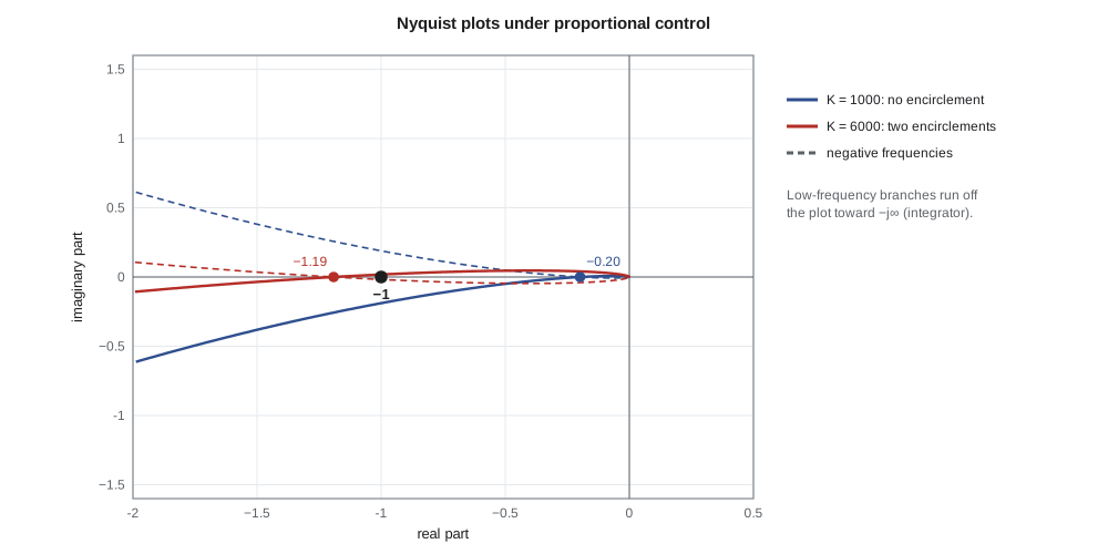
Amara uses the code above to count encirclements numerically for the proportional loop at two gains, tracing the full contour including the small detour round the origin. At K = 1000 V/rad there are no encirclements and, since P = 0, the loop is stable. At K = 6000 V/rad there are two, so two closed-loop poles lie in the right half plane, exactly as the Routh array of lesson 5 found. The point where the plot crosses the negative real axis is the phase crossover, and the distance from that point to −1 is another view of the gain margin: the plot for K = 1000 crosses at about −0.2, so the gain could be raised by a factor of five, 14 dB, to about 5000 V/rad.
Delay, exactly
Frequency-domain methods handle pure delay without approximation, because e^{−jωθ} has magnitude one and phase −ωθ. The cabinet loop with proportional gain K_c has L(jω) = 0.1K_c e^{−j90ω}/(j3000ω + 1). With K_c = 150 W/K, the code finds a crossover at 5.0 mrad/s, a phase margin of 68° and a gain margin of 11 dB, with no Padé approximation needed. Doubling the gain to 300 W/K cuts the gain margin to 4.9 dB and the phase margin to 40°, because the crossover moves to a higher frequency where the delay's phase lag is twice as large. Delay always limits the achievable crossover frequency: a common rule is that ω_c should not exceed about 1/(2θ) if a reasonable phase margin is to be kept, here about 5.6 mrad/s, a closed-loop time constant of a few minutes.
Worked problem
Margins from a Bode reading
Leo's measured open-loop response of the PT-1 with the lead-lag controller shows |L| = 0 dB at 21 rad/s, where the phase is −124°, and a phase of −180° at 240 rad/s, where |L| = −31 dB. Find the margins, estimate the overshoot and settling time, and compare with the model.
Show solution
- Phase margin: 180° − 124° = 56°; gain margin: 31 dB.
- ζ ≈ PM/100 ≈ 0.56, so overshoot ≈ e^{−π × 0.56/√(1 − 0.31)} ≈ 12 %.
- Settling time ≈ 8/ω_c to 10/ω_c = 0.38 to 0.48 s by the rule of thumb; the rule is conservative for this design, whose settling lesson 8 simulated as 0.21 s.
- The model predicted 59.6° and 38 dB; the measurement shows slightly more lag, which lesson 10 attributes to sampling and computation delay.
Answer: PM ≈ 56°, GM ≈ 31 dB and roughly 12 % overshoot: close to the model, with about 4° of extra lag at crossover.
Reading closed-loop behaviour from the loop
The loop gain's Bode plot carries more information than the margins. Where |L| ≫ 1, at low frequency, the closed loop T = L/(1 + L) is close to one and the output follows the reference closely, while the sensitivity S = 1/(1 + L) ≈ 1/L is small, so disturbances at those frequencies are strongly rejected. The lead-lag design has |L| = 58 dB at 0.1 rad/s, so slow wind changes are reduced by a factor of about 800. Where |L| ≪ 1, at high frequency, T ≈ L is small, so sensor noise is not passed to the output, while S ≈ 1, so disturbances there are not reduced at all. The crossover region in between is where the loop's behaviour is decided, and where the phase margin keeps |1 + L| from becoming small. If 1 + L is small at some frequency, S is large there and the loop amplifies disturbances: a peak in |S| above one is the frequency-domain signature of a lightly damped loop.
This view is the basis of loop shaping, the subject of lesson 10. The designer wants high gain at low frequency for accuracy and disturbance rejection, low gain at high frequency for noise rejection and robustness to unmodelled dynamics, and a crossover with enough phase margin, typically with the magnitude falling at about −20 dB/decade through 0 dB. Bode's gain-phase relationship, which holds for minimum-phase systems with no right-half-plane zeros or delay, says that a slope of −20 dB/decade sustained over a decade or so corresponds to a phase near −90°, which gives a phase margin near 90°; a slope of −40 dB/decade corresponds to −180° and no margin at all. A loop must therefore cross over on a −20 dB/decade slope.
Common mistakes
MistakeReading gain margin at the gain crossover.
InsteadGain margin is read at the phase crossover, where the phase is −180°.
MistakeTrusting margins from a model that leaves out delay and sampling.
InsteadUnmodelled lag erodes phase margin; measure the loop or include the delays.
MistakeApplying Z = N + P without counting open-loop unstable poles.
InsteadP is the number of right-half-plane open-loop poles; an unstable plant needs counterclockwise encirclements to be stabilized.
MistakeForgetting the detour round open-loop poles on the imaginary axis.
InsteadAn integrator's detour maps to a large semicircle that closes the Nyquist plot.
Summary and key terms
- The frequency response L(jω) gives gain and phase at each frequency and can be measured on hardware.
- Bode plots add the straight-line contributions of each factor; the pan plant falls at −20, then −40, then −60 dB/decade.
- Gain margin is 1/|L| at the phase crossover; phase margin is 180° plus the phase at the gain crossover.
- The lead-lag pan loop crosses over at 22.1 rad/s with 59.6° of phase margin and a very large modelled gain margin.
- The Nyquist criterion Z = N + P counts closed-loop right-half-plane poles from encirclements of −1; it handles delay and unstable plants rigorously.
- Delay adds phase −ωθ and limits the crossover frequency to about 1/(2θ); the cabinet with K_c = 150 W/K has 68° of phase margin and 11 dB of gain margin.
- Frequency response
- A transfer function evaluated at s = jω, giving gain and phase versus frequency.
- Bode plot
- Plots of magnitude in decibels and phase in degrees against log frequency.
- Gain crossover frequency
- The frequency at which |L(jω)| = 1.
- Phase crossover frequency
- The frequency at which ∠L(jω) = −180°.
- Gain margin
- The factor by which loop gain can rise before instability, 1/|L(jω₁₈₀)|.
- Phase margin
- The additional phase lag at crossover that would bring the loop to the edge of stability.
- Nyquist plot
- The image of the Nyquist contour under L(s), used to count encirclements of −1.
- Argument principle
- The count of encirclements of the origin equals zeros minus poles enclosed by a contour.
Practice problems
Work each problem on paper first, then reveal the answer to check.
A loop has |L| = 1 at 15 rad/s where its phase is −140°. What is the phase margin and the approximate damping?
Show answer
40°; ζ ≈ 0.4.
At the phase crossover, |L| = 0.25. What is the gain margin in decibels?
Show answer
20 log 4 = 12 dB.
What phase does a delay of 0.5 ms add at 100 rad/s?
Show answer
−0.05 rad = −2.9°.
An open-loop stable plant's Nyquist plot encircles −1 once clockwise. How many closed-loop unstable poles are there?
Show answer
Z = N + P = 1 + 0 = 1.
Estimate the cabinet's maximum useful crossover frequency for its 90 s delay.
Show answer
About 1/(2 × 90) = 5.6 mrad/s.
Why must a loop cross over on a slope of about −20 dB/decade?
Show answer
By Bode's gain-phase relation that slope corresponds to roughly −90° of phase, leaving a healthy phase margin; −40 dB/decade leaves almost none.
Lesson quiz · 5 questions
Score 60% or more to complete this lesson.
Create a free account to save your progress, take quizzes and earn a certificate.