Time response of first- and second-order systems

The specifications in lesson 1 were written in terms of a step response: how fast the camera gets to a new angle, how far it overshoots and how long it takes to settle. To design for them, an engineer needs to know how those quantities depend on the closed-loop poles. This lesson works that out for first- and second-order systems, where the relations are exact and simple, and then asks when a higher-order loop behaves like a second-order one. The answer, dominant poles, is the basis of the root-locus design method in lessons 7 and 8.

First-order systems

A first-order system with time constant τ and DC gain K has the transfer function K/(τs + 1) and a single pole at −1/τ. Its unit step response is K(1 − e^{−t/τ}). After one time constant the output has covered 63.2 % of its final change, after three time constants 95 %, and after four 98.2 %. There is no overshoot. The rise time from 10 % to 90 % is 2.2τ, and the 2 % settling time is about 4τ. The pole's distance from the origin, 1/τ, is a direct measure of speed.

The CC-1 cabinet is first order to a good approximation, with τ = 3000 s. A step of 100 W in heater power raises its temperature by 10 K in the long run, 6.3 K of that in the first 50 minutes, and the cabinet is within 2 % of its new temperature only after about 200 minutes. That slowness is not a problem in itself, since the weather changes slowly too, but it means the loop can never correct a sudden disturbance quickly, and lesson 11 tunes the controller with that in mind.

Second-order systems

The standard second-order form ω_n²/(s² + 2ζω_ns + ω_n²) describes the RLC circuit of lesson 2 and the closed-loop pan servo of lesson 3. Its two poles are at s = −ζω_n ± ω_n√(ζ² − 1). The damping ratio ζ decides their character. For ζ > 1 the poles are real and distinct and the response is overdamped, a slow rise like two first-order systems in series. For ζ = 1 they coincide and the response is critically damped, the fastest without overshoot. For 0 < ζ < 1 they are a complex pair and the response is underdamped: it rises faster, overshoots and rings. For ζ = 0 the poles are on the imaginary axis and the response oscillates forever.

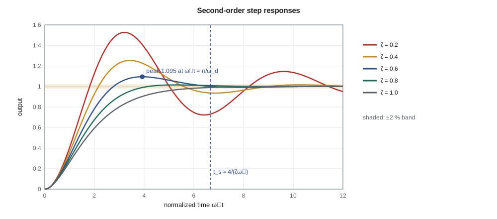
For the underdamped case, the step response has a peak at t_p = π/ω_d, when the sine first reaches the top of its swing. The peak overshoot depends only on ζ: about 53 % at ζ = 0.2, 25 % at 0.4, 9.5 % at 0.6, 4.6 % at 0.7 and 1.5 % at 0.8. The envelope e^{−ζω_nt} sets the settling time: the response stays within 2 % of its final value once the envelope falls below about 0.02, which gives the widely used approximation t_s ≈ 4/(ζω_n). The rise time from 10 % to 90 % has no exact closed form; a good fit for 0.3 < ζ < 0.8 is t_r ≈ (1 − 0.4167ζ + 2.917ζ²)/ω_n.

Specifications as regions of the s-plane

Each specification corresponds to a region in the complex plane where the closed-loop poles must lie. The overshoot depends only on ζ, and ζ = cos β, where β is the angle between the pole and the negative real axis, so a maximum overshoot becomes a wedge: poles must lie within an angle β = arccos ζ_min of the negative real axis. The settling time depends only on the real part ζω_n, so a maximum settling time becomes a vertical line: poles must lie to the left of −4/t_s. The rise time depends mainly on ω_n, the distance from the origin, so a maximum rise time becomes a circle: poles must lie outside radius ω_n,min.

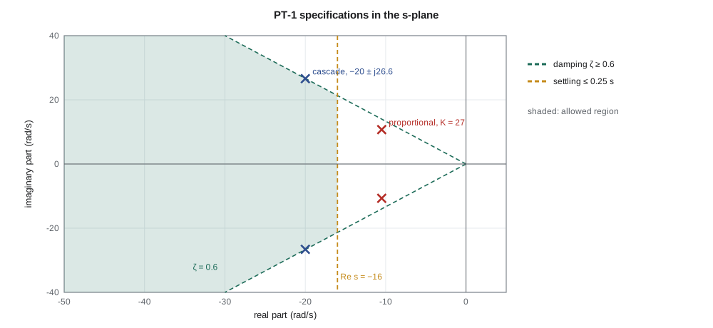
For the PT-1 the specifications of overshoot below 10 % and settling within 0.25 s become ζ ≥ 0.6, a wedge of half-angle 53°, and ζω_n ≥ 4/0.25 = 16 rad/s. Amara's proportional design of lesson 3, with poles at −10.5 ± j10.7, is well damped, ζ = 0.70, but too slow: its real part is −10.5, to the right of −16. The cascade design, with poles at −20 ± j26.6, sits inside the region with ζ = 0.60 and ζω_n = 20.

Checking the formulas

The formulas are exact for a pure second-order system with no zeros. Real loops have extra poles, such as the PT-1's electrical pole at −1979 rad/s, and sometimes zeros. Amara simulates the step responses of four versions of the pan servo and compares the measured specifications with the formulas.

import math
def step_metrics(num, den, t_end=1.0, dt=1e-5):
    """Step response of num/den (highest power first) by RK4 on the controllable canonical form."""
    n = len(den) - 1; a = [c / den[0] for c in den]; b = [0.0] * (n + 1 - len(num)) + [c / den[0] for c in num]
    x = [0.0] * n
    def f(x):  # x[0] is the lowest derivative
        dx = x[1:] + [1.0 - sum(a[n - i] * x[i] for i in range(n))]
        return dx
    def y(x):  # strictly proper numerator: output is a weighted sum of the states
        return sum(b[n - i] * x[i] for i in range(n))
    t, ys = 0.0, []
    while t < t_end:
        k1 = f(x); k2 = f([xi + dt / 2 * k for xi, k in zip(x, k1)])
        k3 = f([xi + dt / 2 * k for xi, k in zip(x, k2)]); k4 = f([xi + dt * k for xi, k in zip(x, k3)])
        x = [xi + dt / 6 * (p + 2 * q + 2 * r + w) for xi, p, q, r, w in zip(x, k1, k2, k3, k4)]
        t += dt; ys.append((t, y(x)))
    yf = ys[-1][1]
    peak = max(v for _, v in ys)
    t10 = next(t for t, v in ys if v >= 0.1 * yf); t90 = next(t for t, v in ys if v >= 0.9 * yf)
    ts = max((t for t, v in ys if abs(v - yf) > 0.02 * yf), default=0.0)
    return (peak / yf - 1) * 100, (t90 - t10), ts
def formulas(zeta, wn):
    Mp = 100 * math.exp(-math.pi * zeta / math.sqrt(1 - zeta**2))
    return Mp, (1 - 0.4167 * zeta + 2.917 * zeta**2) / wn, 4 / (zeta * wn)
cases = [("P, Kp = 27", [224.9], [1, 21, 224.9]),
         ("rate + position", [1108.0], [1, 40, 1108]),
         ("same, with electrical pole", [1108.0 * 1979], [1, 40 + 1979, 1108 + 40 * 1979, 1108 * 1979]),
         ("PD in forward path (zero at -27.7)", [40.0, 1108.0], [1, 40, 1108])]
for name, num, den in cases:
    Mp, tr, ts = step_metrics(num, den)
    print(f"{name:35s} overshoot {Mp:5.1f} %, rise {tr*1000:5.1f} ms, 2 % settling {ts*1000:5.0f} ms")
for zeta, wn in ((0.70, math.sqrt(224.9)), (0.60, math.sqrt(1108))):
    Mp, tr, ts = formulas(zeta, wn)
    print(f"formulas zeta {zeta:.2f}, wn {wn:5.1f}: overshoot {Mp:5.1f} %, rise {tr*1000:5.1f} ms, settling {ts*1000:4.0f} ms")
# first-order cabinet: time to reach 63 % and 98 % of a step
tau = 3000.0
print(f"cabinet: 63 % at {tau/60:.0f} min, 98 % at {4*tau/60:.0f} min")

P, Kp = 27                          overshoot   4.6 %, rise 141.8 ms, 2 % settling   399 ms
rate + position                     overshoot   9.4 %, rise  55.8 ms, 2 % settling   179 ms
same, with electrical pole          overshoot   9.4 %, rise  55.8 ms, 2 % settling   179 ms
PD in forward path (zero at -27.7)  overshoot  24.8 %, rise  26.8 ms, 2 % settling   206 ms
formulas zeta 0.70, wn  15.0: overshoot   4.6 %, rise 142.5 ms, settling  381 ms
formulas zeta 0.60, wn  33.3: overshoot   9.5 %, rise  54.1 ms, settling  200 ms
cabinet: 63 % at 50 min, 98 % at 200 min

For the two pure second-order cases the simulation matches the formulas closely: 4.6 % overshoot and a rise time of 142 ms for the proportional design, 9.4 % and 56 ms for the cascade. The settling times differ by a few per cent from 4/(ζω_n), which is an envelope approximation; the 2 % band is first entered when a ripple crosses it, so the true value jumps in steps as ζ varies. The simulated cascade settles in 179 ms, inside the 250 ms specification. Adding the electrical pole at −1979 rad/s changes nothing visible, because it is about 60 times farther from the origin than the dominant poles.

The fourth case is instructive. It has the same poles as the cascade, but the derivative action has been moved into the forward path, so the closed loop has a zero at −27.7. The overshoot jumps from 9.4 % to 24.8 % and the rise time halves. The zero adds a scaled derivative of the step response to the response itself, which speeds the rise and lifts the peak. This is why the cascade, which applies the derivative action to the measured angle rather than to the error, gives a cleaner step response than a controller with the same gains in the forward path. Lesson 11 calls this derivative on measurement.

Dominant poles

A higher-order system behaves like a second-order one when a pair of poles is much closer to the imaginary axis than all the others, and no zeros sit near them. The far poles' modes decay much faster and are finished before the dominant pair's response has developed. A common rule is that the other poles should be at least five times farther to the left than the dominant pair's real part. The PT-1's electrical pole easily qualifies. A closed-loop pole and zero that nearly coincide also have little effect, because the zero cancels most of the pole's residue; lesson 8's lag compensator relies on that, leaving a slow but small tail in the response.

When the conditions fail, the second-order formulas are only a guide. A third pole near the dominant pair slows the response and, depending on where it is, can reduce or increase overshoot. A zero near the dominant pair increases overshoot if it is in the left half plane, as in the fourth case above, and causes the response to start in the wrong direction if it is in the right half plane. Simulation is always the final check, and it is cheap.

Responses to other inputs

The step is the standard test because it is easy to generate and it excites every mode, but other inputs matter too. A ramp input represents a steady pan; the next two lessons show that a type-1 loop follows it with a constant lag. An impulse represents a sudden knock, such as a gust or a truck passing under the mast arm, and the impulse response is the derivative of the step response. A sinusoid represents a periodic disturbance, such as the sway of the mast arm in a steady wind, and the response to it is the frequency response of lesson 9. Because the system is linear, the response to any combination of these is the sum of the individual responses.

Finally, specifications are usually checked against a small step, where the system is linear. A large step on the PT-1, say 90°, would demand far more than 24 V from the cascade controller in its first instant: 133 V/rad × 1.57 rad is 209 V. The driver saturates, the response is slower than the linear prediction, and the overshoot can be larger. Practical servos therefore move large distances along a planned trajectory with limited speed and acceleration, and use the linear loop to track that trajectory closely. Lesson 12 designs that profile.