Dynamic models of electrical and electromechanical systems

A controller can only be designed against a model of the plant. The model need not be perfect, since lesson 1 showed that feedback tolerates error, but it must capture the dynamics that matter at the speeds the loop will run. For the PT-1 pan axis that means the motor's armature circuit, the inertia of the rotor and camera head, the gearbox and the friction. For the CC-1 it means the cabinet's heat storage and heat loss. This lesson builds both models from physical laws, shows that they lead to ordinary differential equations of the kind solved in ELE-250, and shows how to linearize a plant that is not linear.

The approach is the same for every physical domain. Identify the elements that store energy, because each one contributes a state variable and an order to the differential equation: an inductor stores magnetic energy in its current, a capacitor stores electric energy in its voltage, a rotating mass stores kinetic energy in its speed and a thermal mass stores heat in its temperature. Then write the element laws and the connection laws, Kirchhoff's laws for circuits, Newton's laws for mechanisms and the conservation of energy for heat, and combine them. Leo's job on the test bench is to measure the parameters the equations need.

Electrical networks

Circuits are the most familiar case. A resistor obeys v = Ri, an inductor v = L di/dt and a capacitor i = C dv/dt. For a series RLC circuit driven by a voltage source, Kirchhoff's voltage law gives L di/dt + Ri + v_C = v_s with i = C dv_C/dt, a second-order equation in v_C. Taking Laplace transforms with zero initial conditions, as in ELE-250, turns each element into an impedance, R, sL and 1/(sC), and the transfer function from source to capacitor voltage follows from the voltage divider.

Every second-order system in this course can be written in the standard form on the right, with natural frequency ω_n and damping ratio ζ. For the RLC circuit, ω_n = 1/√(LC) and ζ = (R/2)√(C/L). Lesson 4 relates these two numbers to the shape of the step response. Operational-amplifier circuits are modelled the same way, using the ideal op-amp rules from ELE-240; that is how analog controllers, such as the lead networks of lesson 8, are built.

Mechanical rotation

For rotating mechanisms the element laws are analogous. An inertia J obeys T = J dω/dt, a viscous friction b gives a torque bω opposing motion, and a torsional spring of stiffness k gives a torque kθ. Newton's second law for rotation says that the net torque on a body equals J dω/dt. The analogy between the domains is exact enough that mechanical systems are sometimes simulated as circuits: torque corresponds to voltage or current, speed to the other, inertia to inductance or capacitance and friction to resistance.

Real mechanisms also have friction that is not viscous. Coulomb friction is a constant torque opposing motion, and stiction is a larger torque that must be overcome to start moving. Both are nonlinear and both matter for a camera that must hold still and then move by a fraction of a degree. The linear model here keeps only the viscous term, and lesson 11 returns to what Coulomb friction and stiction do to a loop with integral action.

The DC motor

A permanent-magnet brushed DC motor couples an electrical circuit to a rotating mass. The armature has resistance R and inductance L. When the rotor turns at speed ω, the conductors moving through the magnet's field generate a back-emf e = K_e ω that opposes the applied voltage. The current i in the field produces a torque T = K_t i. In SI units, conservation of energy requires K_t = K_e: the electrical power e·i absorbed by the back-emf equals the mechanical power T·ω delivered. Datasheets often give K_e in volts per thousand rpm and K_t in ounce-inches or newton-metres per ampere, so it is worth converting both and checking that they agree.

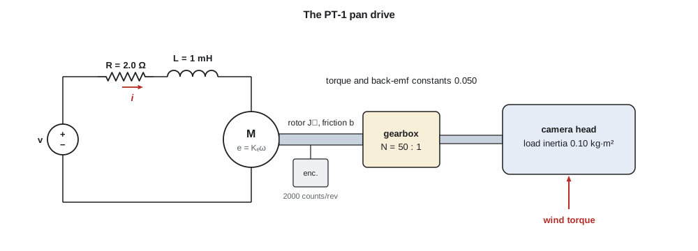
The gearbox multiplies torque by the ratio N and divides speed by N. Seen from the motor shaft, a load inertia J_L looks like J_L/N², because the motor must accelerate the load N times more slowly but through a lever N times longer. A 0.10 kg·m² camera head behind a 50:1 gearbox therefore appears at the motor as only 4.0 × 10⁻⁵ kg·m², comparable to the rotor's own 2.0 × 10⁻⁵ kg·m². This is the usual reason for gearing a servo: it matches a small, fast motor to a large, slow load. A disturbance torque at the camera, such as wind, appears at the motor divided by N.

Taking Laplace transforms and eliminating the current gives the transfer function from voltage to motor speed. Its denominator is a quadratic whose two roots are the poles of the drive. When the electrical time constant L/R is much shorter than the mechanical one, which is almost always true for small motors, the two poles are well separated: a slow mechanical pole set by the inertia and the back-emf, and a fast electrical pole near −R/L.

The mechanical time constant τ_m deserves a closer look. Without back-emf, the motor's speed would be limited only by the tiny friction b, and τ_m would be J/b, several seconds. The back-emf acts like a very strong viscous friction of K_tK_e/R: as the motor speeds up, its back-emf reduces the current and the torque. That electrical damping, not the bearings, sets how quickly the motor reaches speed.

The PT-1 parameters

Leo measures the prototype motor. With the rotor locked, a small DC voltage and an ammeter give R = 2.0 Ω, and a quick current step at the same time gives L ≈ 1.0 mH from the 0.5 ms current rise. Spinning the motor with a drill and measuring its open-circuit voltage gives K_e = 0.050 V·s/rad, or 5.2 V per thousand rpm, which agrees with the datasheet's torque constant of 0.050 N·m/A. The rotor inertia comes from the datasheet, the camera head's from the mechanical drawing, and a run-down test, letting the motor coast from speed with the leads open, gives the small viscous friction. Amara computes the model.

import math
# PT-1 pan axis: armature, motor, gearbox and camera head
R, L = 2.0, 1.0e-3            # armature resistance (ohm) and inductance (H)
Kt = Ke = 0.050               # torque constant N*m/A = back-emf constant V*s/rad
Jm, N, JL = 2.0e-5, 50, 0.10  # motor inertia, gear ratio, load inertia (kg*m^2)
b = 1.0e-5                    # viscous friction at the motor shaft (N*m*s/rad)
J = Jm + JL / N**2            # load inertia reflected to the motor shaft
print(f"reflected load {JL/N**2:.1e}, total J = {J:.1e} kg*m^2")
# omega/V = Kt / ((L s + R)(J s + b) + Kt^2) = Kt / (a2 s^2 + a1 s + a0)
a2, a1, a0 = L * J, L * b + R * J, R * b + Kt**2
disc = math.sqrt(a1**2 - 4 * a2 * a0)
p1, p2 = (-a1 + disc) / (2 * a2), (-a1 - disc) / (2 * a2)
print(f"poles {p1:.1f} and {p2:.0f} rad/s; time constants {-1000/p1:.1f} ms and {-1000/p2:.3f} ms")
Kdc = Kt / a0
print(f"DC gain {Kdc:.2f} rad/s per volt at the motor, {Kdc/N:.4f} at the camera")
print(f"no-load speed at 24 V: {24*Kdc*60/(2*math.pi):.0f} rpm motor, {24*Kdc/N*180/math.pi:.0f} deg/s camera")
tau_m = R * J / (R * b + Kt**2)
print(f"mechanical time constant R*J/(R*b + Kt^2) = {tau_m*1000:.1f} ms, electrical L/R = {L/R*1000:.2f} ms")
# step of 12 V: full model (current and speed states) versus first-order model
def full(t_end, dt=1e-5, V=12.0):
    i = w = t = 0.0; out = {}
    marks = {0.01, 0.05, 0.10, 0.20}
    while t < t_end - 1e-12:
        di = (V - R * i - Ke * w) / L
        dw = (Kt * i - b * w) / J
        i += dt * di; w += dt * dw; t += dt
        for m in marks:
            if abs(t - m) < dt / 2: out[m] = (i, w)
    return out
res = full(0.2)
for t in sorted(res):
    i, w = res[t]
    w1 = 12 * Kdc * (1 - math.exp(-t / tau_m))
    print(f"t = {t*1000:4.0f} ms: current {i:5.2f} A, speed {w:6.1f} rad/s (first-order model {w1:6.1f})")
print(f"starting current 12/R = {12/R:.1f} A; stall torque at camera {Kt*12/R*N:.0f} N*m")
# tilt axis: gravity torque m*g*d*sin(theta), linearized about theta0
m, g, d = 3.5, 9.81, 0.030
for th0 in (0, 30, 60):
    k = m * g * d * math.cos(math.radians(th0))
    print(f"tilt {th0:2d} deg: holding torque {m*g*d*math.sin(math.radians(th0)):.2f} N*m, linear stiffness {k:.2f} N*m/rad")

reflected load 4.0e-05, total J = 6.0e-05 kg*m^2
poles -21.2 and -1979 rad/s; time constants 47.1 ms and 0.505 ms
DC gain 19.84 rad/s per volt at the motor, 0.3968 at the camera
no-load speed at 24 V: 4547 rpm motor, 546 deg/s camera
mechanical time constant R*J/(R*b + Kt^2) = 47.6 ms, electrical L/R = 0.50 ms
t =   10 ms: current  4.97 A, speed   43.4 rad/s (first-order model   45.1)
t =   50 ms: current  2.15 A, speed  154.8 rad/s (first-order model  154.8)
t =  100 ms: current  0.78 A, speed  209.3 rad/s (first-order model  208.9)
t =  200 ms: current  0.13 A, speed  234.6 rad/s (first-order model  234.5)
starting current 12/R = 6.0 A; stall torque at camera 15 N*m
tilt  0 deg: holding torque 0.00 N*m, linear stiffness 1.03 N*m/rad
tilt 30 deg: holding torque 0.52 N*m, linear stiffness 0.89 N*m/rad
tilt 60 deg: holding torque 0.89 N*m, linear stiffness 0.52 N*m/rad

The two poles are at −21.2 rad/s and −1979 rad/s, time constants of 47.1 ms and 0.505 ms, separated by a factor of nearly 100. The first-order model with τ_m = 47.6 ms tracks the full model within a few per cent after the first 10 ms, and is indistinguishable from it after 50 ms. For designing a loop that settles in a quarter of a second, the first-order model is adequate for speed, and the electrical pole matters only when the loop is pushed toward high bandwidth, as lessons 5 and 7 show. The DC gain is 19.84 rad/s per volt at the motor, or 0.3968 rad/s per volt at the camera, and at 24 V the camera can turn at about 546°/s, far faster than any operator needs.

The simulation also shows the starting current. At the instant 12 V is applied the motor is stationary, there is no back-emf and the current rises toward 12/2 = 6 A before the speed builds and pulls it down. At 24 V it would approach 12 A. The motor driver must either tolerate that or limit it, and the controller must not command full voltage reversals casually. These limits return in lesson 11.

From speed to position

The pan angle at the camera is the integral of the camera speed, θ = ω/N integrated, which in the Laplace domain is a division by s. The plant from motor voltage to camera angle is therefore the motor's speed transfer function divided by Ns. That integrator matters enormously: a position servo built on a DC motor has a pole at the origin, which lesson 6 shows gives zero steady-state error to step commands even with simple proportional control.

This is the model Amara carries through the course. Where the electrical pole matters, she uses the full form, 16 667/(s(s + 21.2)(s + 1979)), obtained by dividing K_t/N by LJ and factoring the quadratic. The two forms agree at low frequency, as they should.

Thermal systems: the cabinet

Heat flow has the same structure. A thermal capacitance C, in joules per kelvin, stores heat: C dT/dt equals the net heat flow in. A thermal resistance R_th, in kelvins per watt, carries heat in proportion to a temperature difference. The cabinet's walls, louvres and gaskets together have a conductance UA = 1/R_th of about 10 W/K, and its contents a capacitance of about 30 kJ/K. With the heater power Q as input, the internal dissipation P and the outdoor temperature T_a as disturbances, the cabinet's equation is first order.

This is the electrical RC circuit again, with temperature as voltage and heat flow as current. The real cabinet is not one lump: the air warms in minutes, the steel and batteries in tens of minutes, and heat takes time to reach the sensor. Rather than model every lump, control engineers often fit a first-order-plus-dead-time model to a measured step response, a gain, a time constant and a delay. Lesson 11 does exactly that for the CC-1, with a delay of about 90 s.

Linearization

Many plants are nonlinear. The PT-1's tilt axis is an example. The camera's centre of gravity sits about 30 mm in front of the tilt axis, so gravity exerts a torque mgd sin θ that depends on the tilt angle. The heater in the cabinet is another: if its power were controlled by varying its voltage, the power would vary as V². Transfer functions describe linear systems only, so the standard approach is to linearize about an operating point: write each nonlinear function as its value at the operating point plus the first term of its Taylor series, and keep only the small deviations.

For the tilt axis, with m = 3.5 kg, g = 9.81 m/s² and d = 30 mm, the code above gives the holding torque and the linearized stiffness at three tilt angles. The constant part of the gravity torque is a steady disturbance that the motor must hold; the slope acts like a torsional spring of stiffness mgd cos θ₀, about 1.03 N·m/rad at level and half that at 60° down. Because the stiffness changes with angle, a controller designed at one operating point behaves slightly differently at another. A well designed loop has enough margin that this does not matter, and lesson 10 checks it. When the variation is large, controllers are sometimes scheduled, with gains that change with the operating point.

Linear models are valid for small deviations. A motor driver that saturates at ±24 V, an encoder that counts in steps of 0.0036° and a gearbox with a little backlash are all nonlinear in ways that no Taylor series removes. The linear design comes first because it gives insight and a starting point, and the nonlinear effects are then checked by simulation, as in lessons 11 and 12.

Checking a model

A model should be checked against measurements before it is trusted. Leo applies a 12 V step to the motor on the bench and records the encoder; the measured speed at 50 ms is within 3 % of the model's 155 rad/s, which is as good as the parameter measurements. He also checks that the steady speed scales with voltage, which confirms that the friction is small and the motor nearly linear above a volt or so. Below about 0.4 V the motor does not turn at all, because the starting current cannot overcome stiction, which is the first hint of the nonlinear friction that lesson 11 addresses.