
ELE-390 · Lesson 1 of 12 · 26 min
Introduction to feedback control
Cedarline Controls in Fredericton has spent the last few years building electronics for intersections: the APS-2 accessible pedestrian push-button station, the inductive loop detectors and the TLR-1 telemetry radio. This year the company is taking on two products that move things rather than measure them. The first is the PT-1 pan-tilt unit, a motorized mount that lets a traffic operations centre aim a detection camera on a mast arm from a desk 10 km away. The second is the CC-1 cabinet climate controller, which keeps the steel signal cabinet at the corner warm enough in a New Brunswick winter for its battery backup to deliver its rated runtime. Amara Osei, now an engineer-in-training with three years at the company, leads the control design for both. Daniel Fortin, P.Eng., reviews her work, and Leo Tremblay, a co-op student, builds the test rigs.
Both products have the same problem at their core. Something must be made to behave as commanded, the camera must point where the operator asks and the cabinet must stay at its set temperature, even though the hardware is imperfect, the parameters are uncertain and the weather keeps pushing back. The answer in both cases is feedback: measure what is actually happening, compare it with what is wanted, and use the difference to drive the actuator. This course is about designing those loops so that they are fast, accurate, well damped and, above all, stable. This first lesson introduces the vocabulary, shows with a simple simulation why feedback works, and sets out the specifications that the rest of the course will learn to meet.
Open-loop and closed-loop control
An open-loop controller computes its output from the command alone. A toaster's timer, a washing machine's fixed cycle and a stepper motor driven by counted pulses are open loop: they never check the result. Open-loop control is cheap, needs no sensor and cannot become unstable on its own, but it works only as well as the designer's knowledge of the system. If the bread is thicker, the load heavier or the motor misses steps, the result is wrong and nothing corrects it.
A closed-loop, or feedback, controller measures the controlled quantity and acts on the error between the command and the measurement. The standard picture has six elements. The reference r is the command, such as a pan angle of 35° or a cabinet temperature. The controller computes a signal from the error e = r − y. The actuator, such as a motor driver or a heater relay, turns that signal into physical action. The plant is the thing being controlled: the camera mount with its motor and gearbox, or the cabinet with its air, steel and electronics. The sensor, an encoder or a thermistor, measures the output y. Disturbances d, such as wind torque on the camera or a cold gust through the cabinet louvres, push the output away from where it should be, and sensor noise n corrupts the measurement.
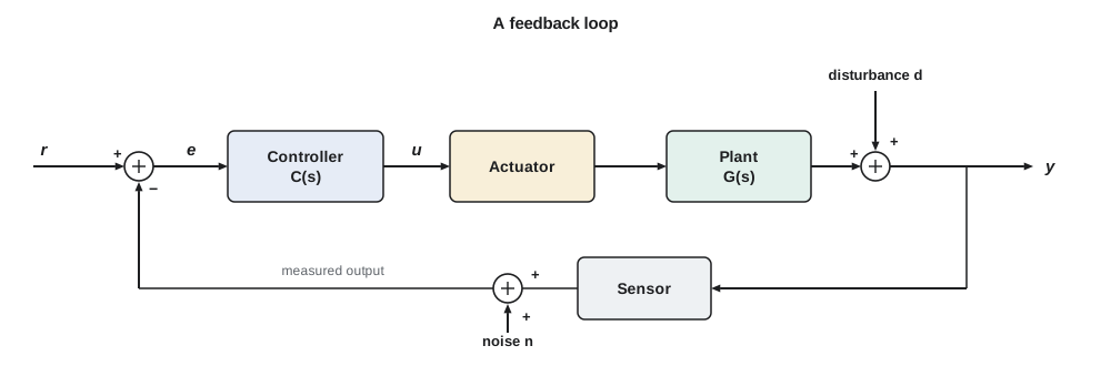
The power of the arrangement is that the controller does not need to know why the output is wrong. Whether the camera lags because the gearbox is stiff on a cold morning, because a gust is pushing on its housing or because the motor's magnet is weaker than the datasheet says, the error appears and the controller responds. Feedback converts a problem of knowing the plant exactly into a problem of measuring the output well, and measuring is usually much easier.
Why feedback works: the cabinet heater
Amara's first sketch for the CC-1 makes the point concretely. A typical steel cabinet at a Fredericton intersection loses heat to the outdoors at about 10 W for every kelvin of difference between inside and outside, and its air, steel, batteries and electronics store about 30 kJ for each kelvin of temperature rise, so its thermal time constant is 30 000/10 = 3000 s, or 50 minutes. The electronics inside dissipate about 120 W. A 400 W heater must hold the inside at 10 °C, where the battery backup's lead-acid cells keep most of their capacity, when it is −30 °C outside. The temperature sensor sits in a small housing on the door, and between the heater, the air mixing and the housing there is an effective delay of about 90 s before a change in heat shows up in the reading.
She compares three strategies in a simple simulation. In open loop, the heater is set to the fixed power that balances the losses on a design day, 280 W. In on-off control, a thermostat switches the full 400 W on when the reading falls 1 K below the set point and off when it rises 1 K above. In proportional control, the heater power is proportional to the error, 150 W for each kelvin below the set point, limited to the range 0 to 400 W. Each strategy is tested on the design day, on a milder day and on a design day when the electronics are idle and dissipate only 40 W.
# Traffic cabinet heater: open-loop setting versus on-off and proportional feedback
C, UA = 30000.0, 10.0                    # J/K, W/K
Q_max, delay = 400.0, 90.0                # heater W, sensor lag s
Tset = 10.0
def run(mode, Ta, P_int=120.0, hours=6.0, dt=1.0, Kp=150.0, fixed=280.0, band=1.0):
    T, heater_on, hist = Tset, False, [Tset] * int(delay / dt)
    temps = []
    for k in range(int(hours * 3600 / dt)):
        Tm = hist[0]                           # what the delayed sensor reads
        if mode == 'open':
            Q = fixed
        elif mode == 'onoff':
            if Tm < Tset - band: heater_on = True
            if Tm > Tset + band: heater_on = False
            Q = Q_max if heater_on else 0.0
        else:
            Q = min(Q_max, max(0.0, Kp * (Tset - Tm)))
        T += dt * (Q + P_int - UA * (T - Ta)) / C
        hist = hist[1:] + [T]
        temps.append(T)
    last = temps[-3600:]
    return min(last), max(last), sum(last) / len(last)
for Ta, Pi in ((-30.0, 120.0), (-20.0, 120.0), (-30.0, 40.0)):
    print(f"outdoor {Ta:.0f} C, electronics {Pi:.0f} W")
    for mode in ('open', 'onoff', 'prop'):
        lo, hi, avg = run(mode, Ta, Pi)
        print(f"  {mode:6s}: last hour {lo:5.1f} to {hi:5.1f} C, mean {avg:5.1f} C")
# sensitivity of the closed loop to a 20 % drop in the heater's output
for Kp in (50.0, 150.0, 400.0):
    L = Kp / UA
print(f"Kp = {Kp:.0f} W/K: loop gain {L:.0f}, steady error for -30 C {(UA*(Tset+30) - 120.0)/(UA + Kp):.2f} K, S = {1/(1+L):.3f}")outdoor -30 C, electronics 120 W open : last hour 10.0 to 10.0 C, mean 10.0 C onoff : last hour 8.2 to 11.3 C, mean 9.8 C prop : last hour 8.2 to 8.2 C, mean 8.2 C outdoor -20 C, electronics 120 W open : last hour 20.0 to 20.0 C, mean 20.0 C onoff : last hour 8.5 to 11.6 C, mean 10.0 C prop : last hour 8.9 to 8.9 C, mean 8.9 C outdoor -30 C, electronics 40 W open : last hour 2.0 to 2.0 C, mean 2.0 C onoff : last hour 8.0 to 11.1 C, mean 9.8 C prop : last hour 7.7 to 7.7 C, mean 7.7 C Kp = 50 W/K: loop gain 5, steady error for -30 C 4.67 K, S = 0.167 Kp = 150 W/K: loop gain 15, steady error for -30 C 1.75 K, S = 0.062 Kp = 400 W/K: loop gain 40, steady error for -30 C 0.68 K, S = 0.024
The open-loop heater is perfect on the day it was calibrated for, holding exactly 10.0 °C. On a −20 °C day it overheats the cabinet to 20 °C, wasting about 100 W around the clock, and when the electronics go idle on a cold night it lets the cabinet sink to 2 °C, where the batteries lose much of their capacity. Nothing in the open-loop controller notices. The on-off thermostat holds the mean near 10 °C in every case, but it cycles between about 8 °C and 11.5 °C; the 90 s delay means the temperature keeps falling after the heater switches on and keeps rising after it switches off, so the swing is wider than the 2 K band. The proportional controller holds a steady temperature without cycling, but it settles below the set point, at 8.2 °C, 8.9 °C and 7.7 °C in the three cases.
That residual error is not a flaw in the simulation; it is how proportional control works. A proportional controller produces heat only when there is an error, so to deliver the 280 W the cabinet needs on the design day it must sit about 1.75 K below the set point. Raising the gain shrinks the offset, to 0.68 K at 400 W/K, but in a loop with delay a high gain eventually causes oscillation, as lesson 5 will show. Lesson 6 explains how integral action removes the offset entirely, and lesson 11 tunes the CC-1's final controller.
The algebra of feedback
The cabinet results follow from a few lines of algebra that apply to every loop in this course. Suppose the controller and plant together have a gain L, the loop gain, from error to output. With the loop closed, y = L e and e = r − y, so y = L(r − y), or y/r = L/(1 + L). If L is large, y/r is close to 1 whatever the exact value of L. A disturbance d added at the output gives y = d/(1 + L) when r = 0, so it is reduced by the factor 1 + L. Two functions capture this and appear throughout the course: the sensitivity function S = 1/(1 + L) and the complementary sensitivity T = L/(1 + L), which add to one.
The last relation is the reason for the sensitivity function's name. A fractional change in the loop gain, from a weak motor magnet, a heater element that has aged or a battery voltage that has sagged, produces a fractional change in the closed-loop gain that is smaller by the factor S. With a loop gain of 15, a 20 % drop in heater output changes the closed-loop gain by only 20 % × 1/16, or 1.25 %. Harold Black used exactly this argument in the 1920s for the negative-feedback amplifier, as ELE-340 described: trade surplus gain for precision. In a control loop the gains are functions of frequency, and lesson 9 shows that S and T can be shaped separately at different frequencies.
Worked problem
Sensitivity of the proportional cabinet loop
The proportional cabinet controller has a gain of 150 W/K, and the cabinet loses 10 W/K. Treat the loop gain at steady state as L = 150/10 = 15. The heater's output falls by 20 % as it ages. By how much does the closed-loop steady-state gain change, and how does that compare with open-loop control?
Show solution
- The closed-loop gain from set point to temperature is T = L/(1 + L).
- \[T = \frac{15}{16} = 0.9375 \qquad T' = \frac{12}{13} = 0.9231\]
- The fractional change is (0.9231 − 0.9375)/0.9375 = −1.5 %, close to the small-change estimate S × (−20 %) = −1.25 %.
- An open-loop heater would deliver 20 % less heat, and the cabinet's rise above ambient would fall by 20 %.
Answer: The closed-loop gain changes by about 1.5 %, compared with 20 % in open loop: feedback reduces the effect by roughly the factor 1 + L.
What feedback costs
Feedback is not free. It needs a sensor, and the loop can be no better than the measurement: the controller faithfully follows sensor errors, so a thermistor that reads 2 K high holds the cabinet 2 K too cold, and encoder noise appears as motor current. The noise term in the figure enters with the same transfer function as the reference, T, so a loop with a high gain at high frequencies passes sensor noise straight to the actuator. Feedback also needs an actuator with spare capacity: when the heater is already at 400 W the loop has no more authority, and no gain can help.
Most importantly, feedback can make a system unstable. The cabinet's 90 s delay means that the controller always acts on old information. With a modest gain, the corrections arrive late but small. With a large gain, the corrections are large and late, so the controller overcorrects, then overcorrects the other way, and the temperature oscillates with growing amplitude. The same happens in the pan-tilt unit, where the motor's inductance, the shaft's inertia and the controller's sampling all add lag. Stability is the first requirement of every loop, and lessons 5, 7 and 9 give three ways to test it.
The PT-1 pan axis
The pan-tilt unit is the course's main design problem. Its pan axis is driven by a 24 V brushed DC motor through a 50:1 gearbox. An incremental encoder on the motor shaft, with 500 lines read in quadrature, gives 2000 counts per motor revolution and so 100 000 counts per revolution of the camera, a resolution of 0.0036°. A microcontroller samples the encoder and updates the motor drive every millisecond. The camera head and its weatherproof housing add inertia, and the housing catches the wind.
The traffic operations centre's specification, which Amara turns into engineering terms over the next eleven lessons, is short. An operator who clicks on a new aim point expects the camera to get there quickly and stop without visible overshoot; when the camera is following a slow pan across an intersection, the image must not lag behind the commanded path; and a gust must not knock the view off its target. For small moves she writes: settle to within 2 % of a 10° step in 0.25 s with no more than 10 % overshoot, follow a 20°/s pan with an error of no more than 0.2°, and hold position against a steady wind torque. She adds two requirements that the operators never mention but every control engineer would: the loop must remain stable with margin when the motor and load parameters vary, and the motor voltage must stay within the driver's ±24 V.
| Requirement | Engineering specification | Where it is treated |
|---|---|---|
| Gets there quickly | 2 % settling time ≤ 0.25 s for a 10° step | Lessons 4, 7, 8 |
| Stops cleanly | Overshoot ≤ 10 %, so damping ratio ζ ≥ 0.6 | Lessons 4, 8 |
| Follows a slow pan | Ramp error ≤ 0.2° at 20°/s, so velocity constant K_v ≥ 100 s⁻¹ | Lesson 6 |
| Holds against wind | Zero steady error for a constant disturbance torque | Lessons 6, 11, 12 |
| Robust | Phase margin ≥ 50°, gain margin ≥ 10 dB | Lessons 9, 10 |
| Within hardware limits | Motor voltage within ±24 V; 1 kHz sampling | Lessons 11, 12 |
Kinds of control problems
The two Cedarline products illustrate the two broad kinds of control problems. The cabinet is a regulator: its reference rarely changes, and the job is to reject disturbances, the outdoor temperature and the changing electronic load. The pan axis is mostly a servomechanism, or servo: its reference changes often, and the job is to track it. The same tools serve both, but the emphasis differs. Regulators are judged by how well they reject disturbances and how little energy they waste; servos by their speed and accuracy in following commands.
Control problems also differ by how the controller is built. The cabinet's on-off thermostat is a nonlinear controller with only two outputs; the proportional controller is linear until the heater saturates. Most of this course treats linear time-invariant models, because they can be analyzed with the transfer functions and frequency responses of ELE-250 and give results that carry over well to real hardware near an operating point. Lesson 2 shows how to linearize a nonlinear plant, and lessons 11 and 12 return to the nonlinear facts of life: saturation, quantization and sampling.
A short history
Feedback control is older than electronics. James Watt's centrifugal governor of the 1780s regulated steam-engine speed by opening the throttle as the engine slowed, and engineers soon found that governors could hunt, oscillating instead of settling. James Clerk Maxwell's 1868 paper on governors was one of the first mathematical stability analyses. The modern theory took shape in the telephone industry: Black's feedback amplifier in the late 1920s, Nyquist's stability criterion in 1932 and Bode's work on gain and phase in the 1940s, all at Bell Laboratories. Ziegler and Nichols published their famous tuning rules for industrial controllers in 1942, and Walter Evans introduced the root locus in 1948. From about 1960 the state-space methods associated with Rudolf Kalman added a matrix description suited to computers and to systems with many inputs and outputs. This course follows that order: transfer functions and the root locus, then frequency response, then an introduction to state space.
How control engineers specify a loop
Specifications fall into a few families, and each has a precise meaning that later lessons develop. Transient-response specifications describe the step response: rise time, peak overshoot and settling time, which lesson 4 relates to pole locations. Steady-state specifications give the error left after transients die away for steps, ramps or constant disturbances, which lesson 6 relates to the number of integrators in the loop. Stability margins, the gain and phase margins of lesson 9, say how much the plant can change before the loop goes unstable. Bandwidth says over what range of frequencies the output follows the reference. Effort limits bound the actuator's output, which matters because a design that meets every other specification by demanding 200 V from a 24 V driver is not a design.
These specifications pull against each other. A faster response needs more actuator effort and more bandwidth, which admits more sensor noise; a higher gain improves accuracy but erodes stability margins. Much of control engineering is managing those trade-offs, and good specifications say what matters most. For the PT-1, Daniel's review note is blunt: an operator will forgive a camera that takes a tenth of a second longer to arrive, but not one that rings or drifts in the wind.
Common mistakes
MistakeAssuming feedback fixes a poor sensor.
InsteadThe loop follows the measurement, errors and all; the sensor sets the accuracy limit.
MistakeRaising the gain until the steady error is small enough.
InsteadHigh gain in a loop with lag leads to oscillation and instability; integral action removes steady error without unlimited gain.
MistakeIgnoring actuator limits in the design.
InsteadA saturated actuator breaks the loop; check the effort the design demands.
MistakeJudging an on-off thermostat by its switching band.
InsteadDelay makes the actual temperature swing wider than the band.
Summary and key terms
- Open-loop control acts on the command alone and cannot correct for disturbances or plant changes; closed-loop control acts on the measured error.
- The loop elements are reference, controller, actuator, plant, sensor, disturbance and noise.
- With loop gain L, the closed loop is T = L/(1 + L) and the sensitivity is S = 1/(1 + L); disturbances and plant changes are reduced by about 1 + L.
- Proportional control leaves a steady error; on-off control cycles; integral action, introduced in lesson 6, removes steady error.
- Feedback needs a good sensor and actuator headroom, and it can cause instability when the loop contains lag.
- Specifications cover transient response, steady-state error, stability margins, bandwidth and actuator effort, and they trade off against each other.
- Open-loop control
- Control computed from the command alone, without measuring the output.
- Closed-loop control
- Control that measures the output and acts on the error between command and measurement.
- Plant
- The system being controlled, including its actuator dynamics when convenient.
- Loop gain
- The product of the transfer functions around the feedback loop, L = CG.
- Sensitivity function
- S = 1/(1 + L), the factor by which feedback reduces disturbances and the effect of plant changes.
- Complementary sensitivity
- T = L/(1 + L), the closed-loop transfer function from reference to output.
- Regulator
- A control system whose main job is to hold a constant output against disturbances.
- Servomechanism
- A control system whose main job is to track a changing reference.
Practice problems
Work each problem on paper first, then reveal the answer to check.
A loop has L = 50. By what factor does feedback reduce a constant output disturbance?
Show answer
1 + L = 51.
The cabinet proportional gain is raised to 300 W/K. Find the steady error on the design day.
Show answer
(10 × 40 − 120)/(10 + 300) = 280/310 = 0.90 K.
A closed-loop gain must vary by no more than 1 % when the plant gain varies by 25 %. What loop gain is needed?
Show answer
S ≤ 0.04, so 1 + L ≥ 25 and L ≥ 24.
Why does the on-off thermostat swing wider than its switching band?
Show answer
The 90 s delay means the heater's effect continues to build, or decay, after each switch.
Classify the CC-1 and the PT-1 as regulators or servomechanisms.
Show answer
The CC-1 is mainly a regulator; the PT-1 is mainly a servomechanism.
What camera angle does one encoder count represent?
Show answer
360°/(2000 × 50) = 0.0036°.
Lesson quiz · 5 questions
Score 60% or more to complete this lesson.
Create a free account to save your progress, take quizzes and earn a certificate.