
ELE-390 · Lesson 7 of 12 · 22 min
The root locus
The Routh criterion tells the designer where a loop stops being stable. It does not show where the closed-loop poles are on the way, and lesson 4 showed that their exact location decides the step response. In 1948 Walter Evans, working on aircraft guidance, published a graphical method that shows exactly that: the root locus, the path traced in the s-plane by the closed-loop poles as one gain varies from zero to infinity. A sketch of the locus, made in minutes with a few rules, shows at a glance whether a specification can be met by adjusting gain and, if not, what kind of compensator would help. This lesson develops the rules and applies them to the PT-1 pan servo, with a result that explains why Amara's proportional designs could never settle fast enough.
The angle and magnitude conditions
Write the loop gain as KG(s), where K ≥ 0 is the gain being varied and G(s) = N(s)/D(s) contains everything else. The closed-loop poles are the roots of 1 + KG(s) = 0, or KG(s) = −1. A complex number equals −1 when its magnitude is one and its angle is an odd multiple of 180°. Because K is real and positive, these split into two conditions. The angle condition says a point s is on the locus if and only if the angle of G(s) is 180° plus a multiple of 360°. The magnitude condition then gives the gain that puts a closed-loop pole there.
The angle condition does not involve K at all. That is the key insight: the shape of the locus depends only on the open-loop poles and zeros, and the gain merely says where on the locus the closed-loop poles sit. Each term in the angle condition can be drawn as a vector from a pole or zero to the trial point, so the test is geometric. A designer with a protractor, or a few lines of code, can decide whether any point is on the locus and, if not, by how many degrees it misses.
Rules for sketching
Evans's rules follow from the two conditions and from the behaviour of the polynomial D(s) + KN(s) at the extremes of K. With n open-loop poles and m zeros, the main rules are these.
| Rule | Statement |
|---|---|
| Number of branches | n branches, one for each closed-loop pole; the locus is symmetric about the real axis. |
| Start and end | Branches start at the open-loop poles (K = 0) and end at the open-loop zeros or at infinity (K → ∞). |
| Real axis | A real-axis point is on the locus if the number of real poles and zeros to its right is odd. |
| Asymptotes | n − m branches go to infinity along asymptotes at angles (2k + 1)180°/(n − m), meeting the real axis at the centroid σ = (Σp − Σz)/(n − m). |
| Breakaway points | Where branches leave or join the real axis, dK/ds = 0. |
| Imaginary-axis crossings | Found from the Routh array or by substituting s = jω into the characteristic equation. |
| Departure and arrival angles | At a complex pole or zero, the angle condition applied to a point very close to it gives the direction of the branch. |
The real-axis rule is the angle condition in disguise. A complex pair of poles or zeros contributes equal and opposite angles to a real-axis point and so cancels, and real poles or zeros to the left contribute 0°, so only those to the right matter, each contributing 180°. The asymptote rule describes the locus far from all the poles and zeros, where it looks as if n − m poles were concentrated at the centroid. For n − m = 1 the single asymptote is the negative real axis; for 2 it is a vertical line through the centroid; for 3 it is three lines at ±60° and 180°.
The pan servo under proportional control
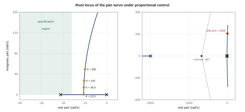
Amara applies the rules to the PT-1 pan axis with the full plant of lesson 2, KG(s) = 16 667K/(s(s + 21.2)(s + 1979)). There are three poles and no zeros, so three branches, all going to infinity.
The real-axis segments are from 0 to −21.2, where there is one pole to the right, and to the left of −1979, where there are three. The three asymptotes leave the centroid (0 − 21.2 − 1979)/3 = −666.7 at angles of +60°, −60° and 180°. The branches starting at 0 and −21.2 move toward each other, meet at a breakaway point and leave the real axis as a complex pair; the branch from −1979 moves left along the real axis forever. The breakaway point satisfies dK/ds = 0, where K = −s(s + 21.2)(s + 1979)/16 667. The complex pair heads up and down, bending slowly to the right toward the ±60° asymptotes, and crosses the imaginary axis at the frequency and gain lesson 5 found.
import math, cmath
def roots(p, iters=400):
    a = [c / p[0] for c in p]; n = len(a) - 1
    z = [(0.4 + 0.9j) ** k * 100 for k in range(n)]
    f = lambda x: sum(c * x ** (n - i) for i, c in enumerate(a))
    for _ in range(iters):
        z = [zi - f(zi) / math.prod(zi - zj for j, zj in enumerate(z) if j != i) for i, zi in enumerate(z)]
    return sorted(z, key=lambda r: (round(r.real, 6), r.imag))
# open loop K * 16667 / (s (s + 21.2)(s + 1979)): den = s^3 + 2000.2 s^2 + 41975 s
den = [1.0, 2000.2, 21.2 * 1979.0, 0.0]; g = 16667.0
poles = [0.0, -21.2, -1979.0]
# asymptotes: n - m = 3 branches to infinity
centroid = sum(poles) / 3
print(f"asymptote centroid {centroid:.1f}, angles 60, 180, 300 deg")
# breakaway: dK/ds = 0 with K = -den(s)/g  ->  3 s^2 + 4000.4 s + 41975 = 0
a, b, c = 3.0, 2 * 2000.2, 21.2 * 1979.0
sb = (-b + math.sqrt(b * b - 4 * a * c)) / (2 * a)
Kb = -(sb**3 + 2000.2 * sb**2 + 21.2 * 1979.0 * sb) / g
print(f"breakaway at s = {sb:.2f}, gain {Kb:.2f} V/rad")
# imaginary-axis crossing from the Routh condition
print(f"j-axis crossing at {math.sqrt(21.2 * 1979.0):.0f} rad/s, gain {2000.2 * 21.2 * 1979.0 / g:.0f} V/rad")
# walk along the locus and report damping and settling estimates
print("   K     dominant poles        zeta   4/(zeta wn)   third pole")
for K in (5.0, 13.3, 20.0, 36.8, 100.0, 300.0, 1000.0, 4000.0):
    r = roots([1.0, 2000.2, 21.2 * 1979.0, g * K])
    dom = max(r, key=lambda x: x.real); third = min(r, key=lambda x: x.real)
    wn = abs(dom); zeta = -dom.real / wn
    print(f"{K:6.1f}  {dom.real:8.2f} ± j{abs(dom.imag):6.2f}   {zeta:5.2f}   {4/(zeta*wn)*1000:7.0f} ms   {third.real:8.1f}")
# angle condition check at a trial point: the point -20 + j26.6 is not on the locus
s0 = complex(-20, 26.6)
ang = -sum(math.degrees(cmath.phase(s0 - p)) for p in poles)
print(f"angle of G at -20 + j26.6: {ang:.1f} deg (a locus point needs -180); shortfall {(-180 - ang):.1f} deg")asymptote centroid -666.7, angles 60, 180, 300 deg breakaway at s = -10.57, gain 13.27 V/rad j-axis crossing at 205 rad/s, gain 5035 V/rad K dominant poles zeta 4/(zeta wn) third pole 5.0 -2.22 ± j 0.00 1.00 1801 ms -1979.0 13.3 -10.57 ± j 0.50 1.00 378 ms -1979.1 20.0 -10.56 ± j 7.55 0.81 379 ms -1979.1 36.8 -10.52 ± j 14.11 0.60 380 ms -1979.2 100.0 -10.39 ± j 27.10 0.36 385 ms -1979.4 300.0 -9.96 ± j 49.25 0.20 402 ms -1980.3 1000.0 -8.46 ± j 91.28 0.09 473 ms -1983.3 4000.0 -2.14 ± j182.75 0.01 1867 ms -1995.9 angle of G at -20 + j26.6: -215.1 deg (a locus point needs -180); shortfall 35.1 deg
The breakaway point is at −10.57, reached when K = 13.3 V/rad. From there the dominant pair rises almost straight up, its real part creeping from −10.6 to −10.4 as K rises to 100 and to −8.5 at 1000. Damping falls steadily: ζ = 0.6 at K = 36.8, 0.36 at 100, 0.09 at 1000. The settling-time estimate 4/(ζω_n) = 4/|real part| barely changes from 380 ms until the pair begins to bend toward the imaginary axis, and the electrical pole meanwhile wanders from −1979 to −1996, never close enough to matter.
The conclusion is the most useful thing a root locus can tell a designer: no value of proportional gain meets the specification. The settling requirement needs the dominant poles to the left of −16, and the dominant branches never get there. Raising the gain only adds oscillation. This is not a matter of tuning; it is a matter of where the open-loop poles are. The branches leave the real axis halfway between the poles at 0 and −21.2, and with no zeros nearby to pull them left, they stay there.
Testing a desired pole location
Lesson 3's cascade design put the closed-loop poles at −20 ± j26.6, inside the specification region. The angle condition shows how far that point is from the proportional locus. The angle of G at s₀ = −20 + j26.6 is −(126.9° + 87.4° + 0.8°) = −215.1°, the three terms being the angles of the vectors from the poles at 0, −21.2 and −1979. A point on the locus needs −180°, so the point misses by 35.1°. A compensator that adds 35.1° of phase at s₀ would put the locus through it. That is exactly what the lead compensator of lesson 8 does, and the number 35.1° is its design target.
The rate loop of lesson 3 reached the point a different way. Feeding back speed changed the plant the outer loop sees, moving its pole from −21 to −40, and with the poles at 0 and −40 the breakaway point moves to −20. The proportional locus for that modified plant rises vertically through −20, and K_p = 133 V/rad places the pair at ±j26.6. Root locus thinking explains the cascade too: the designer chose K_d to move the open-loop pole, then chose K_p to slide along the new locus.
Worked problem
Root locus of PI position control
Sketch the locus of the pan servo with PI control C(s) = K(s + 5)/s using the reduced plant 8.33/(s(s + 21)). Find the real-axis segments, the asymptotes and the gain at which the locus crosses the imaginary axis, if it does.
Show solution
- The loop gain is 8.33K(s + 5)/(s²(s + 21)): poles at 0, 0 and −21, a zero at −5, so n − m = 2.
- Real-axis segment: between −5 and −21 (three poles and zeros to the right: 0, 0 and −5). Asymptotes at ±90° through σ = (0 + 0 − 21 − (−5))/2 = −8.
- The double pole at the origin splits into a pair leaving at ±90° and bending toward the vertical asymptotes at −8; the branch from −21 moves right to end at the zero.
- \[s^3 + 21s^2 + 8.33Ks + 41.7K = 0;\quad 21 \times 8.33K > 41.7K \text{ for all } K > 0\]
Answer: The locus never crosses into the right half plane: the integral zero at −5 lies to the right of the motor pole at −21, which lesson 5 showed is the condition T_i = 0.2 s > 0.0476 s. The dominant poles approach the asymptotes at Re s = −8, too slow for the specification without further compensation.
Other uses of the locus
The locus need not be drawn against a controller gain. Any parameter that enters the characteristic equation linearly can be isolated: rewrite the equation as 1 + αG′(s) = 0 and draw the locus of the new G′ against α. Daniel uses this to check the effect of the camera head's inertia. The PT-1 will be sold with two housings, the standard one and a heated version with a larger window that adds 40 % to the load inertia, and the locus against inertia shows the cascade's poles moving toward the imaginary axis by a few degrees, comfortably inside the specification region. A locus against a sensor time constant or a delay approximation answers similar questions.
The locus also extends to negative K, the complementary root locus, which describes positive feedback or a plant whose gain changes sign. It appears when a sensor is wired with the wrong polarity, a classic commissioning error. With the encoder's A and B channels swapped, the PT-1's feedback becomes positive, the complementary locus puts one closed-loop pole in the right half plane at any gain, and the camera spins away until it reaches a limit. Leo's commissioning checklist starts by jogging the motor open loop and confirming that the encoder counts in the right direction.
Software and judgement
Computers draw loci accurately in milliseconds, and the code above simply finds the roots at many gains. The value of the sketching rules is not in drawing but in reasoning. A designer who knows that branches bend toward zeros, that asymptotes depend on n − m and that poles near the origin dominate the response can look at a plant and say, before any computation, that proportional control will be too slow, that a zero is needed to pull the locus left, and roughly where to put it. That reasoning is the subject of lesson 8.
Common mistakes
MistakeReading the step response from the gain alone.
InsteadFind where that gain places the poles on the locus, then apply the lesson 4 relations.
MistakeApplying the real-axis rule counting only poles.
InsteadCount both poles and zeros to the right of the point.
MistakeForgetting that branches with n − m ≥ 3 eventually cross into the right half plane.
InsteadThree or more asymptotes always include lines at less than 90° from the positive real axis.
MistakeAssuming a higher gain always gives a faster response.
InsteadOn the pan servo's locus the real part barely changes; only the oscillation increases.
Summary and key terms
- The root locus is the path of the closed-loop poles as a gain K varies from 0 to ∞.
- A point is on the locus if the angle of G(s) is an odd multiple of 180°; the gain there is 1/|G(s)|.
- Branches start at open-loop poles and end at zeros or along n − m asymptotes from the centroid.
- Real-axis segments lie to the left of an odd number of real poles and zeros; breakaway points satisfy dK/ds = 0.
- For the pan servo, the dominant branches break away at −10.6 and rise almost vertically, so proportional control cannot reach the required real part of −16.
- The desired point −20 + j26.6 misses the locus by 35.1°, which sets the phase a compensator must add.
- Root locus
- The set of closed-loop pole locations as a gain varies from zero to infinity.
- Angle condition
- A point is on the locus if ∠G(s) = ±180°(2k + 1).
- Magnitude condition
- The gain placing a pole at s is K = 1/|G(s)|.
- Asymptote
- A straight line that n − m branches approach as K → ∞.
- Centroid
- The point (Σp − Σz)/(n − m) on the real axis where the asymptotes meet.
- Breakaway point
- A real-axis point where branches leave or join the axis.
- Departure angle
- The direction in which a branch leaves a complex open-loop pole.
- Complementary root locus
- The locus for negative gain, describing positive feedback.
Practice problems
Work each problem on paper first, then reveal the answer to check.
For KG(s) = K/(s(s + 4)), find the breakaway point and the gain there.
Show answer
dK/ds = 0 gives s = −2; K = 4.
Find the asymptote centroid and angles for K(s + 3)/(s(s + 1)(s + 5)(s + 10)).
Show answer
n − m = 3; σ = (−16 + 3)/3 = −4.33; ±60° and 180°.
Is s = −3 on the locus of K/(s(s + 2)(s + 5))?
Show answer
No: two poles, at 0 and −2, lie to its right, an even number.
What gain on the pan locus gives ζ = 0.7?
Show answer
About 27 V/rad, the lesson 3 proportional design.
How many degrees must a compensator add for the locus to pass through −20 + j26.6?
Show answer
35.1°.
Why does the electrical pole barely move along the locus up to K = 1000 V/rad?
Show answer
It is far from the other poles; its branch heads left along the real axis slowly.
Lesson quiz · 5 questions
Score 60% or more to complete this lesson.
Create a free account to save your progress, take quizzes and earn a certificate.