PID tuning and digital implementation

The PID controller is the workhorse of practical control. Surveys of process plants have long found that the large majority of their loops are PID or PI, and the same is true of the motor drives, power supplies and thermostats in everyday equipment. Its popularity comes from its three terms' clear meanings, proportional for the present error, integral for the accumulated past and derivative for the predicted future, and from the fact that it can be tuned by experiment without a detailed model. This lesson tunes the CC-1 cabinet controller from a step test, deals with what happens when the heater saturates, and then turns to how any continuous controller, the PT-1's lead-lag included, is implemented as a few lines of code that run at a fixed sampling rate.

Forms of the PID controller

The textbook, or ideal, form is u = K_c[e + (1/T_i)∫e dt + T_d de/dt], with controller gain K_c, integral time T_i and derivative time T_d. The parallel form writes the same thing with independent gains, u = K_Pe + K_I∫e dt + K_D de/dt, where K_I = K_c/T_i and K_D = K_cT_d. Older analog controllers used a series, or interacting, form, K_c′(1 + 1/(T_i′s))(1 + T_d′s), which is the lead-PI structure of lesson 8; its settings convert to the ideal form, and tuning rules always say which form they assume.

Practical controllers modify the ideal form in three ways. The derivative is filtered, as above, with N typically between 5 and 20, so that its gain at high frequency is limited to N times K_c; lesson 10 explained why. The derivative is usually applied to the measurement rather than the error, −T_d dy/dt instead of T_d de/dt, so that a step in the set point does not produce a spike in the output; lesson 4 showed the overshoot that derivative on the error causes, and lesson 3's rate loop is exactly derivative on measurement. The proportional term may act on a weighted error, b·r − y with 0 ≤ b ≤ 1, which reduces overshoot to set-point changes without changing the response to disturbances. These modifications make the PID a two-degree-of-freedom controller, in which the responses to commands and to disturbances can be adjusted separately.

Tuning from a step test

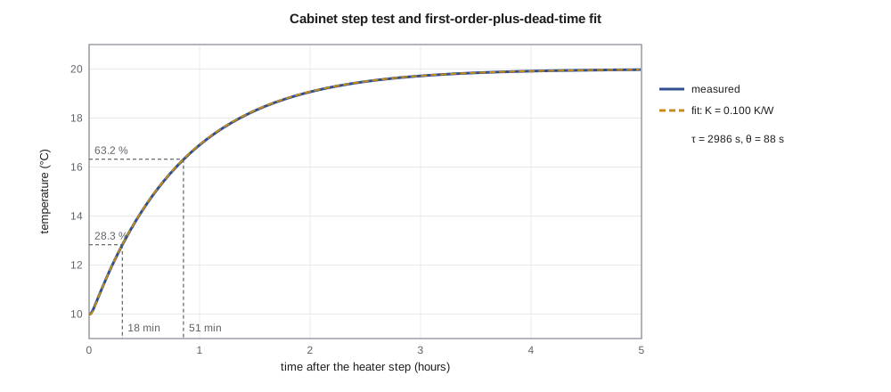
Many plants, the cabinet among them, are well described for tuning purposes by a first-order-plus-dead-time model, K e^{−θs}/(τs + 1), whose three parameters can be read from an open-loop step test. With the cabinet steady at 10 °C on a cold night and the heater at 280 W, Leo steps the heater to 380 W and logs the temperature for five hours. The gain is the final change divided by the step. A simple two-point method gives the other two: find the times t₂₈ and t₆₃ at which the response has covered 28.3 % and 63.2 % of its final change; then τ = 1.5(t₆₃ − t₂₈) and θ = t₆₃ − τ. The method works because a first-order response reaches those fractions at θ + τ/3 and θ + τ.

Two families of tuning rules then give the PI settings. The Ziegler–Nichols reaction-curve rules of 1942, K_c = 0.9τ/(Kθ) and T_i = 3.33θ, were chosen to give a quarter-amplitude decay ratio, a fast response that many engineers now regard as too aggressive. The SIMC rules published by Sigurd Skogestad in 2003 add a single tuning parameter, the desired closed-loop time constant τ_c, and give K_c = τ/(K(τ_c + θ)) and T_i = min(τ, 4(τ_c + θ)). Choosing τ_c = θ gives a robust, well-damped loop with a gain margin of about 3 and a phase margin of about 47° for a pure first-order-plus-dead-time plant; a smaller τ_c gives a faster, less robust loop.

Integrator windup

Every real actuator saturates. The cabinet heater cannot deliver more than 400 W or less than 0 W, and the PT-1 driver cannot exceed ±24 V. When the actuator is saturated the loop is effectively open: the error persists, the integral term keeps integrating it, and the controller's internal state grows far beyond anything the actuator can deliver. When the error finally reverses, the integral term must unwind before the output leaves saturation, and the result is a large overshoot and a slow recovery. This is integrator windup, and it happens whenever a large disturbance or set-point change drives the actuator to its limit.

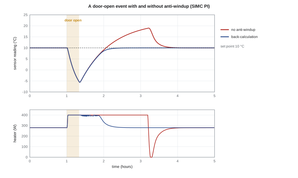
The CC-1's worst case is a winter maintenance visit. A technician opens the cabinet door at −30 °C for 20 minutes, which roughly triples the heat loss. The heater goes to 400 W and stays there, the temperature falls, and the integral term keeps accumulating error. Anti-windup schemes stop that accumulation. The simplest, conditional integration or clamping, freezes the integrator while the output is saturated and the error would drive it further. Back-calculation feeds the difference between the saturated and unsaturated outputs back into the integrator, bleeding it toward a value consistent with the limit. Amara simulates the visit with both tunings, with and without back-calculation.

import math
temp = lambda c: f"{c:.1f} C"          # display helpers
dtemp = lambda d: f"{d:.2f} K"
# "true" cabinet: one thermal mass, a sensor housing that lags by a minute, and a 30 s transport delay
C, UA, tau_s, delay = 30000.0, 10.0, 60.0, 30.0
def cabinet(Q_of_t, Ta_of_t, UA_of_t=lambda t: UA, t_end=6 * 3600, dt=1.0, T0=10.0, Ts=10.0, ctrl=None):
    T = Tsen = T0; buf = [T0] * int(delay / dt); out = []; Q = 0.0
    for k in range(int(t_end / dt)):
        t = k * dt
        meas = Tsen
        if ctrl and k % int(Ts / dt) == 0: Q = ctrl(t, meas)
        elif not ctrl: Q = Q_of_t(t)
        T += dt * (Q + 120.0 - UA_of_t(t) * (T - Ta_of_t(t))) / C
        buf = buf[1:] + [T]
        Tsen += dt * (buf[0] - Tsen) / tau_s
        out.append((t, meas, Q))
    return out
# 1. step test: heater from 280 W to 380 W at t = 0, outdoor -30 C, starting from steady state
base = 10.0
step = cabinet(lambda t: 380.0, lambda t: -30.0, t_end=5 * 3600)
y0 = step[0][1]; yinf = step[-1][1]
def t_at(frac):
    return next(t for t, y, _ in step if y - y0 >= frac * (yinf - y0))
t28, t63 = t_at(0.283), t_at(0.632)
K = (yinf - y0) / 100; tau = 1.5 * (t63 - t28); theta = t63 - tau
print(f"step test: 28.3 % at {t28:.0f} s, 63.2 % at {t63:.0f} s -> K = {K:.3f} K/W, tau = {tau:.0f} s, theta = {theta:.0f} s")
# 2. tuning rules for a PI controller
zn = (0.9 * tau / (K * theta), 3.33 * theta)          # Ziegler-Nichols reaction curve
tc = theta                                              # SIMC with closed-loop time constant = theta
simc = (tau / (K * (tc + theta)), min(tau, 4 * (tc + theta)))
for name, (Kc, Ti) in (("Ziegler-Nichols", zn), ("SIMC", simc)):
    print(f"{name:16s}: Kc = {Kc:5.0f} W/K, Ti = {Ti:5.0f} s")
# 3. a winter maintenance visit: door open 20 min (UA x 3), then closed; PI with and without anti-windup
def make_pi(Kc, Ti, antiwindup, Ts=10.0, sp=10.0, qmax=400.0):
    st = {'I': 280.0}
    def ctrl(t, y):
        e = sp - y
        u = Kc * e + st['I']
        u_sat = min(qmax, max(0.0, u))
        if not antiwindup or u == u_sat:
            st['I'] += Kc * Ts / Ti * e                  # integrate normally
        else:
            st['I'] += (u_sat - u) * 0.5 + 0.0          # back-calculation: bleed the integrator toward the limit
        return u_sat
    return ctrl
door = lambda t: UA * (3.0 if 3600 <= t < 3600 + 1200 else 1.0)
for Kc, Ti in (zn, simc):
    for aw in (False, True):
        out = cabinet(None, lambda t: -30.0, UA_of_t=door, ctrl=make_pi(Kc, Ti, aw), t_end=9 * 3600)
        after = [y for t, y, _ in out if t > 3600 + 1200]
        low = min(y for t, y, _ in out); high = max(after)
        settle = max((t for t, y, _ in out if t > 4800 and abs(y - 10) > 0.5), default=4800) - 4800
        print(f"Kc {Kc:4.0f}, Ti {Ti:4.0f}, anti-windup {str(aw):5s}: low {temp(low)}, peak after door {temp(high)}, "
              f"back within 0.5 K after {settle/60:3.0f} min")
# 4. a sudden 5 K drop in outdoor temperature (heater stays within its range)
for name, (Kc, Ti) in (("Ziegler-Nichols", zn), ("SIMC", simc)):
    out = cabinet(None, lambda t: -35.0, ctrl=make_pi(Kc, Ti, True), t_end=4 * 3600)
    ys = [y for _, y, _ in out]
    dip = min(ys); k = ys.index(dip); over = max(ys[k:])
    print(f"{name:16s}: falls {dtemp(10 - dip)} below set point, then rises {dtemp(max(0.0, over - 10))} above it")

step test: 28.3 % at 1084 s, 63.2 % at 3075 s -> K = 0.100 K/W, tau = 2986 s, theta = 88 s
Ziegler-Nichols : Kc =   304 W/K, Ti =   295 s
SIMC            : Kc =   169 W/K, Ti =   708 s
Kc  304, Ti  295, anti-windup False: low -5.6 C, peak after door 19.4 C, back within 0.5 K after 177 min
Kc  304, Ti  295, anti-windup True : low -5.6 C, peak after door 10.0 C, back within 0.5 K after  43 min
Kc  169, Ti  708, anti-windup False: low -5.6 C, peak after door 19.0 C, back within 0.5 K after 141 min
Kc  169, Ti  708, anti-windup True : low -5.6 C, peak after door 10.0 C, back within 0.5 K after  49 min
Ziegler-Nichols : falls 0.18 K below set point, then rises 0.02 K above it
SIMC            : falls 0.27 K below set point, then rises 0.00 K above it

The two-point fit gives K = 0.100 K/W, τ = 2986 s and θ = 88 s, close to the values used since lesson 1, although the true plant in the simulation is a thermal mass with a one-minute sensor lag and a 30 s transport delay rather than a pure delay; the fit lumps the lag into θ. Ziegler–Nichols gives K_c = 304 W/K and T_i = 295 s; SIMC with τ_c = θ gives K_c = 169 W/K and T_i = 708 s. During the door-open visit the cabinet falls to −5.6 °C with either tuning, because the heater is saturated and no controller can do more. The difference comes afterward. Without anti-windup, the wound-up integrator holds the heater at full power long after the door closes, and the cabinet overshoots to 19 °C, nine degrees above the set point, taking more than two hours to return. With back-calculation the temperature returns to 10 °C without overshoot, within 0.5 K after 43 to 49 minutes.

For the small, unsaturated disturbance of a sudden 5 K fall in outdoor temperature, the two tunings differ as expected. The more aggressive Ziegler–Nichols loop holds the cabinet within 0.18 K and then overshoots slightly; SIMC lets it fall 0.27 K and recovers without overshoot. Both are far better than the battery backup needs. Amara chooses the SIMC settings for their margins, since the cabinet's parameters vary from site to site with cabinet size, sun exposure and equipment load, and adds back-calculation anti-windup. Daniel's review adds one more requirement: the controller's integrator must be initialized to the current heater output when the CC-1 switches from manual to automatic, so that the switch does not bump the output. That bumpless transfer is the same idea as anti-windup, keeping the integrator consistent with what the actuator is actually doing.

The ultimate-gain method

Ziegler and Nichols also gave a closed-loop method. With integral and derivative action turned off, the proportional gain is raised until the loop oscillates steadily; the gain K_u and the period P_u of that oscillation then set the controller: K_c = 0.45K_u and T_i = P_u/1.2 for PI, or K_c = 0.6K_u, T_i = P_u/2 and T_d = P_u/8 for PID. For the cabinet, lesson 5 found K_u = 530 W/K and P_u = 356 s, which give a PI setting of 238 W/K and 297 s, similar to the reaction-curve result. The method needs no model, but it deliberately drives the plant to the edge of instability, which is acceptable for a cabinet heater on a mild day and not for a camera on a mast arm over traffic. Modern autotuners obtain the same information more gently with relay feedback, switching the actuator between two levels so that the loop settles into a small limit cycle whose amplitude and period give K_u and P_u.

Discrete-time implementation

The PT-1 and the CC-1 both run their controllers on microcontrollers, which sample the measurement every T seconds, compute an output and hold it until the next sample. A continuous controller C(s) must therefore be converted to a difference equation. Three conversions are common. The backward-difference, or backward Euler, method replaces s by (1 − q⁻¹)/T, where q⁻¹ means one sample of delay; it is simple and always gives a stable discrete controller from a stable continuous one. The bilinear, or Tustin, method replaces s by (2/T)(1 − q⁻¹)/(1 + q⁻¹); it maps the imaginary axis onto the unit circle exactly and preserves frequency responses well up to a fraction of the sampling frequency, and it can be prewarped to match one critical frequency exactly, as ELE-250 described for filters. Matched pole-zero mapping places each pole and zero at e^{sT}.

Amara converts the PT-1's lead-lag compensator by Tustin's method at 1 kHz, section by section, and checks the result against the continuous controller's frequency response.

import math
T = 0.001                                        # 1 kHz sampling
def tustin(z, p, w_match=None):
    """(s + z)/(s + p) -> (b0 + b1 q^-1)/(1 + a1 q^-1) by the bilinear transform s = (2/T)(1 - q^-1)/(1 + q^-1)."""
    c = 2 / T
    b0, b1, a0, a1 = c + z, z - c, c + p, p - c
    return b0 / a0, b1 / a0, a1 / a0
sections = [(21.2, 40.0), (0.5, 0.125)]
K = 120.0
for z, p in sections:
    b0, b1, a1 = tustin(z, p)
    print(f"(s + {z})/(s + {p}):  y[k] = {b0:.6f} x[k] {b1:+.6f} x[k-1] {-a1:+.6f} y[k-1]")
# check: discrete and continuous frequency responses agree well below the Nyquist frequency
for w in (1.0, 22.0, 200.0, 1000.0):
    s = 1j * w; q = complex(math.cos(w * T), math.sin(w * T))
    Cc = K; Cd = K
    for z, p in sections:
        Cc *= (s + z) / (s + p)
        b0, b1, a1 = tustin(z, p); Cd *= (b0 + b1 / q) / (1 + a1 / q)
    print(f"w = {w:6.0f} rad/s: continuous {abs(Cc):7.2f} at {math.degrees(math.atan2(Cc.imag, Cc.real)):6.2f} deg, "
          f"discrete {abs(Cd):7.2f} at {math.degrees(math.atan2(Cd.imag, Cd.real)):6.2f} deg")
# fixed-point concern: the lag section's pole is very close to 1
b0, b1, a1 = tustin(0.5, 0.125)
print(f"lag pole in the q-plane {-a1:.7f}; in Q15 format it would round to {round(-a1 * 32768) / 32768:.7f}")

(s + 21.2)/(s + 40.0):  y[k] = 0.990784 x[k] -0.970000 x[k-1] +0.960784 y[k-1]
(s + 0.5)/(s + 0.125):  y[k] = 1.000187 x[k] -0.999688 x[k-1] +0.999875 y[k-1]
w =      1 rad/s: continuous   70.61 at -18.17 deg, discrete   70.61 at -18.17 deg
w =     22 rad/s: continuous   80.33 at  16.27 deg, discrete   80.33 at  16.27 deg
w =    200 rad/s: continuous  118.33 at   5.15 deg, discrete  118.34 at   5.14 deg
w =   1000 rad/s: continuous  119.93 at   1.05 deg, discrete  119.94 at   0.97 deg
lag pole in the q-plane 0.9998750; in Q15 format it would round to 0.9998779

Each first-order section becomes a difference equation with three coefficients, and the discrete controller's frequency response matches the continuous one to within 0.01 in gain and 0.1° in phase up to 200 rad/s; at 1000 rad/s, a sixth of the Nyquist frequency of 3142 rad/s, the phase differs by only 0.08°. The sampling rate is generous: a common rule asks for sampling at 10 to 30 times the closed-loop bandwidth, and 1 kHz is about 280 times the crossover frequency of 22 rad/s, which is 3.5 Hz. The main cost of sampling is the half-sample delay of the zero-order hold, already counted in lesson 10.

The lag section exposes a practical trap. Its discrete pole is at 0.999875, very close to one, because its continuous pole at −0.125 rad/s is so slow compared with the sampling rate. Stored in a 16-bit fixed-point format, that coefficient would round to 0.9998779, which moves the continuous-time pole from 0.125 to 0.122 rad/s. That error is harmless here, but a coefficient that rounded to exactly 1.0 would turn the lag into an integrator, and one that rounded above 1.0 would make the controller unstable. The PT-1 firmware uses 32-bit floating point for the controller states, and Leo's code review checks that every slow pole is represented accurately. The same concern applies to integrators: the integral term should be accumulated in a variable with enough resolution that small errors still change it, or the loop will settle with a small offset.

Friction, quantization and limit cycles

Nonlinearities that are invisible in a linear analysis can make a well-tuned loop misbehave. The PT-1's gearbox has stiction, so a small error produces no motion until the integral term builds enough voltage to break the camera free; it then jumps, overshoots the target, and the process repeats in the other direction. The result is a small, slow oscillation, a hunting limit cycle, of a few encoder counts. The usual remedies are to make the integral action weaker near zero error, to add a small dead band in which the integrator stops, or to compensate the friction by adding a feedforward voltage in the direction of motion. Quantization of the encoder and of the PWM output can cause similar limit cycles. These effects are the subject of nonlinear control and are mostly handled by simulation and testing.