Markets and government: price controls and taxes

Governments intervene in markets in many ways. They cap rents, set minimum wages, tax gasoline, alcohol and tobacco, collect sales taxes on most purchases, and impose tariffs on imports. These policies usually have worthy aims: making housing affordable, raising the incomes of low-paid workers, discouraging harmful consumption or raising revenue for public services. The supply and demand model, combined with the surplus tools of lesson 5, lets us predict their effects, including effects their designers may not intend. This lesson analyses price ceilings, price floors, taxes and tariffs. It is not an argument for or against any particular policy; it is a toolkit for understanding the trade-offs, together with the evidence on how these policies work in practice.

Price ceilings

A price ceiling is a legal maximum price. If the ceiling is set above the equilibrium price, it has no effect; it is not binding. If it is set below equilibrium, it is binding: at the ceiling price, quantity demanded exceeds quantity supplied, and a shortage results. Because the price cannot rise to ration the good, some other mechanism must decide who gets it: waiting lines, first come first served, personal connections, discrimination by sellers, or black markets in which the good is resold illegally at higher prices. Sellers may also reduce quality, since they cannot raise the price and buyers are queuing anyway.

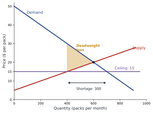
A binding ceiling also creates a deadweight loss. The quantity traded falls from the equilibrium quantity to the smaller quantity that sellers are willing to supply at the ceiling price, so trades that would have benefited both sides do not happen. Some surplus is transferred from sellers to the buyers lucky enough to obtain the good at the low price, but total surplus falls. And if the scarce supply is not allocated to the buyers who value it most, the loss is larger still.

Rent control

Rent control is the most widely debated price ceiling. Economists distinguish first-generation rent control, which freezes rents below market levels, from second-generation rent stabilization, which limits how much rents can rise for sitting tenants, usually allows increases tied to inflation and often exempts new buildings. In the short run, the supply of rental housing is very inelastic, so rent limits mainly transfer income from landlords to tenants with little immediate loss of units. In the long run, supply is more elastic: controls can discourage the construction of new rental buildings, encourage owners to convert units to condominiums or short-term rentals, and reduce spending on maintenance. Controls also reduce mobility, because tenants paying below-market rents are reluctant to move even when their needs change.

In Ontario, rent increases for sitting tenants in units first occupied on or before 15 November 2018 are limited by an annual guideline linked to the consumer price index and capped at 2.5 %; the 2026 guideline is 2.1 %. Units first occupied after that date are exempt from the guideline, a rule intended to protect incentives to build. British Columbia applies its cap to all private rentals; the 2026 maximum allowable increase is 2.3 %, down from 3.0 % in 2025. In both provinces, rent can be reset to market levels when a unit becomes vacant (vacancy decontrol). Manitoba, Quebec, Prince Edward Island and Nova Scotia also regulate increases. Supporters argue that these limits protect tenants from sudden increases and displacement in tight markets; critics argue that they discourage rental construction and maintenance, and that the real problem is too little supply.

The empirical evidence supports parts of both views. A widely cited study by Rebecca Diamond, Tim McQuade and Franklin Qian of San Francisco's 1994 expansion of rent control found that tenants in newly controlled buildings were substantially more likely to stay in their homes, as intended, but that landlords of those buildings reduced the supply of rental housing by about 15 %, through conversions and redevelopment, which pushed up market rents citywide. Studies of Cambridge, Massachusetts, after rent control was abolished in 1995 found increases in property values and investment. Evidence on milder second-generation stabilization with new-construction exemptions suggests smaller supply effects. Most economists favour expanding supply as the main route to affordability, sometimes combined with targeted housing allowances for low-income renters; tenant advocates often favour rent stabilization as protection while supply catches up.

Price floors and the minimum wage

A price floor is a legal minimum price. If it is set above equilibrium, it is binding, and quantity supplied exceeds quantity demanded, creating a surplus. Agricultural price supports have historically created surpluses that governments had to buy, store or export. The most important price floor in modern economies is the minimum wage, a floor on the price of labour. In the simple competitive model, a binding minimum wage raises the wage for workers who keep their jobs but reduces the quantity of labour demanded, causing some unemployment, especially among less experienced workers whose productivity is closest to the minimum.

Canada's federal minimum wage, which applies to federally regulated industries such as banking, telecommunications and interprovincial transportation, rose to $18.15 an hour on 1 April 2026; it is adjusted each year for inflation. Each province and territory sets its own minimum for other workers. Ontario's general minimum wage rose to $17.95 an hour on 1 October 2026, and British Columbia, Nova Scotia and other provinces also index their minimums to inflation. Several cities and advocacy groups calculate a living wage that is considerably higher, reflecting local housing costs.

The evidence on minimum wage effects is one of the most studied questions in economics. In 1994, David Card and Alan Krueger compared fast-food employment in New Jersey, which raised its minimum wage, with neighbouring Pennsylvania, which did not, and found no reduction in employment in New Jersey; Card later shared the 2021 Nobel Prize partly for this work. Their findings were challenged by David Neumark and William Wascher, who found negative effects using other data. More recent studies using many state increases, such as work by Doruk Cengiz, Arindrajit Dube and colleagues, find that moderate increases have had little effect on the number of low-wage jobs while raising earnings, whereas studies of Seattle's rise toward $15 found a reduction in hours worked by low-wage workers. Canadian studies have tended to find modest negative effects on teen employment.

One explanation for small job losses is monopsony, a market with a single or dominant buyer of labour, examined in lesson 12. When employers have wage-setting power, a moderate minimum wage can raise both wages and employment, up to a point. A reasonable summary of current evidence is that moderate minimum wage increases raise earnings for low-wage workers with small employment effects, while very large increases relative to local median wages carry a greater risk of job losses; economists continue to disagree about where that threshold lies.

Taxes

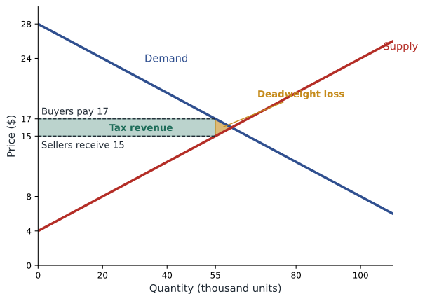
When a government taxes a good, it drives a wedge between the price buyers pay and the price sellers receive. Whether the tax is legally levied on buyers or sellers makes no difference to the outcome: in either case, the price buyers pay rises, the price sellers receive falls, and the quantity traded falls. As lesson 4 showed, the burden is shared according to elasticities, with the less elastic side bearing more. The government collects revenue equal to the tax per unit times the quantity sold after the tax. The fall in quantity creates a deadweight loss, because some trades worth more to buyers than they cost sellers no longer happen.

Deadweight loss grows with the square of the tax. Doubling the tax doubles the wedge and roughly doubles the fall in quantity, so the deadweight-loss triangle, whose area depends on both, roughly quadruples. This is why economists generally prefer broad taxes at low rates to narrow taxes at high rates: a broad-based sales tax or income tax raises a given amount of revenue with less distortion than very high taxes on a few goods. Deadweight loss is also larger when supply and demand are more elastic, because quantity responds more to the tax.

# Revenue and deadweight loss as a per-unit tax rises (linear market from the example)
a, b, c, d = 140, 5, -20, 5
q0 = a - b * (a - c) / (b + d)
print(" tax  quantity  revenue($000)  DWL($000)")
for t in [0, 2, 4, 6, 8, 10, 12, 14, 16]:
    pb = (a - c + d * t) / (b + d)       # price buyers pay
    q = max(a - b * pb, 0)
    revenue = t * q
    dwl = 0.5 * t * (q0 - q)
    print(f"{t:4}  {q:8.1f}  {revenue:13.1f}  {dwl:9.1f}")

 tax  quantity  revenue($000)  DWL($000)
   0      60.0            0.0        0.0
   2      55.0          110.0        5.0
   4      50.0          200.0       20.0
   6      45.0          270.0       45.0
   8      40.0          320.0       80.0
  10      35.0          350.0      125.0
  12      30.0          360.0      180.0
  14      25.0          350.0      245.0
  16      20.0          320.0      320.0

The table illustrates a Laffer-curve pattern for a single market: revenue rises with the tax at first, peaks at a tax of $12 in this example, and would then fall, while deadweight loss rises ever faster. Real tax systems are more complex, but the lesson is general: high tax rates on a narrow base raise little extra revenue at a high cost in lost surplus.

Sales and excise taxes in practice

Canada levies the 5 % federal goods and services tax (GST) on most goods and services. Five provinces (Ontario, New Brunswick, Nova Scotia, Newfoundland and Labrador, and Prince Edward Island) combine it with their provincial sales tax as a harmonized sales tax (HST) of 13 % to 15 %; Quebec applies its own QST alongside the GST; British Columbia, Saskatchewan and Manitoba levy separate provincial sales taxes; and Alberta and the territories levy only the GST. Prices are usually displayed before tax. Canada also levies excise taxes on fuel, alcohol, tobacco, cannabis and vaping products. The consumer carbon charge on fuels was set to zero on 1 April 2025, while carbon pricing for large industrial emitters, through the federal output-based pricing system or equivalent provincial systems, continued, with a federal review of the carbon pricing benchmark in 2026.

Taxes on goods with harmful side effects, such as tobacco, alcohol and carbon emissions, are sometimes called corrective or Pigouvian taxes, after the economist Arthur Pigou. Unlike ordinary taxes, they may improve efficiency rather than reduce it, because they make buyers and sellers take account of costs they would otherwise ignore. Lesson 12 develops this idea.

Tariffs revisited

A tariff is a tax on imports, and the same tools apply. Consider a small country that can import a good at a world price below its domestic equilibrium price. Under free trade, domestic consumers buy at the world price, domestic producers supply what they can profitably make at that price, and imports fill the gap. A tariff raises the domestic price by the amount of the tariff. Consumers lose surplus, domestic producers gain surplus, and the government gains tariff revenue, but two deadweight-loss triangles appear: one because domestic producers with costs above the world price now produce (a production inefficiency), and one because consumers who valued the good above the world price but below the tariff-inclusive price stop buying (a consumption inefficiency). This is the formal basis for the conclusion in lesson 2 that tariffs usually reduce total welfare.