
ECON-101 · Lesson 7 of 12 · 28 min
Consumer choice
Behind every demand curve are millions of individual decisions about how to spend limited incomes. Why does a student buy three coffees a week rather than five? Why do people buy more of most goods when prices fall, and why do some people buy less of certain goods when their incomes rise? The theory of consumer choice answers these questions by modelling how a rational consumer allocates a budget among goods to make herself as well off as possible. It provides the foundation for the law of demand, explains the substitution and income effects introduced in lesson 3, and shows how economists think about the value of goods, the effects of taxes and subsidies, and the design of transfer programs. The lesson ends with behavioural economics, which studies the systematic ways real people depart from the rational model. BUS-220 lesson 4 approached consumer behaviour from a marketer's perspective, with psychology and decision processes; here we use the economist's formal tools.
Utility and marginal utility
Economists use the term utility for the satisfaction or well-being a person gets from consuming goods and services. Utility cannot be measured directly, but it is a useful concept for thinking about choices. Total utility is the overall satisfaction from consuming a given quantity; marginal utility is the extra satisfaction from consuming one more unit. The law of diminishing marginal utility states that, beyond some point, each additional unit of a good brings less extra satisfaction than the one before. The first slice of pizza when you are hungry is wonderful; the fourth is pleasant; the eighth may be unpleasant. Diminishing marginal utility is why people spread their spending across many goods rather than spending everything on one.
| Slices of pizza | Total utility (utils) | Marginal utility (utils) |
|---|---|---|
| 0 | 0 | — |
| 1 | 20 | 20 |
| 2 | 36 | 16 |
| 3 | 48 | 12 |
| 4 | 56 | 8 |
| 5 | 60 | 4 |
| 6 | 60 | 0 |
| 7 | 56 | −4 |
The budget constraint
A consumer's choices are limited by her income and the prices she faces. If she spends her whole income on two goods, X and Y, with prices \( P_X \) and \( P_Y \), her budget constraint is:
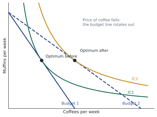
Graphically, the budget line shows all combinations of X and Y she can just afford. Its intercepts are \( I/P_X \) on the X axis and \( I/P_Y \) on the Y axis, and its slope is \( -P_X/P_Y \), the rate at which the market lets her trade Y for X. An increase in income shifts the budget line outward in parallel. A fall in the price of X rotates the line outward around the Y intercept, because she can now buy more X with her income while the maximum amount of Y is unchanged.
Maximizing utility: the equal marginal principle
How should a consumer allocate her budget to maximize total utility? The answer is the equal marginal principle: she should arrange her purchases so that the marginal utility per dollar spent is the same for every good. If the last dollar spent on coffee brings more satisfaction than the last dollar spent on snacks, she can become better off by shifting a dollar from snacks to coffee. As she buys more coffee, its marginal utility falls; as she buys fewer snacks, theirs rises. She should keep shifting until the marginal utilities per dollar are equal.
Worked problem
Allocating a weekly budget
Jordan has $20 a week for coffee ($4 each) and muffins ($2 each). The marginal utilities of successive coffees are 40, 32, 24, 16 and 8 utils; of successive muffins 18, 16, 12, 8, 6, 4, 2 and 1 utils. How should he spend his $20?
Show solution
- Compute marginal utility per dollar. Coffees: 10, 8, 6, 4, 2. Muffins: 9, 8, 6, 4, 3, 2, 1, 0.5.
- Buy in order of highest MU per dollar until the budget is spent: coffee 1 (10), muffin 1 (9), coffee 2 (8), muffin 2 (8), coffee 3 (6), muffin 3 (6).
- Spending so far: 3 × $4 + 3 × $2 = $18. The next best items are coffee 4 (4 per dollar, $4) and muffin 4 (4 per dollar, $2); only $2 remains, so buy muffin 4.
- Total spending: 3 coffees ($12) + 4 muffins ($8) = $20. Marginal utility per dollar of the last units: coffee 6, muffin 4; the next coffee would give 4 per dollar but cannot be afforded.
Answer: Jordan buys 3 coffees and 4 muffins. With whole units the marginal utilities per dollar cannot be equalized exactly, but no feasible reallocation raises his total utility; the code below confirms it by checking every affordable bundle.
# Check every affordable bundle of coffee ($4) and muffins ($2) with a $20 budget
mu_coffee = [40, 32, 24, 16, 8]
mu_muffin = [18, 16, 12, 8, 6, 4, 2, 1]
budget, pc, pm = 20, 4, 2
best = None
for c in range(len(mu_coffee) + 1):
    for m in range(len(mu_muffin) + 1):
        if c * pc + m * pm <= budget:
            u = sum(mu_coffee[:c]) + sum(mu_muffin[:m])
            if best is None or u > best[0]:
                best = (u, c, m)
print(f"best bundle: {best[1]} coffees and {best[2]} muffins, total utility {best[0]} utils")best bundle: 3 coffees and 4 muffins, total utility 150 utils
Deriving the demand curve
The equal marginal principle explains the law of demand. Suppose the price of coffee falls. The marginal utility per dollar of coffee rises, so the consumer buys more coffee until its marginal utility has fallen enough to restore the balance. Tracing the quantity of coffee chosen at each price gives the individual's demand curve, and summing across consumers gives market demand.
A price change has two effects. The substitution effect is the change in quantity demanded caused by the change in relative prices, holding the consumer's level of well-being constant: when coffee becomes cheaper relative to tea, the consumer substitutes toward coffee. The substitution effect always works in the direction predicted by the law of demand. The income effect is the change in quantity demanded caused by the change in purchasing power: a lower price for coffee leaves the consumer with more real income to spend. For a normal good, the income effect reinforces the substitution effect, so a lower price increases quantity demanded. For an inferior good, the income effect works in the opposite direction, but for almost all goods it is too small to outweigh the substitution effect, so demand curves still slope downward.
The theoretical exception is a Giffen good, a strongly inferior good that takes a large share of the budget, for which the income effect outweighs the substitution effect so that quantity demanded rises when price rises. Robert Jensen and Nolan Miller found evidence of Giffen behaviour among very poor households in China's Hunan province in 2008: when the price of rice, their staple, was subsidized, some households bought less rice and more meat, because the subsidy made them feel rich enough to diversify. Giffen goods are rare curiosities, but they illustrate the logic of the two effects.
Indifference curves
A more general approach, which does not require measuring utility in units, uses indifference curves. An indifference curve shows all the combinations of two goods that give the consumer the same level of satisfaction. Indifference curves slope downward, because if the consumer gets less of one good she must get more of the other to stay equally well off. Curves further from the origin represent higher satisfaction. And indifference curves are usually bowed inward toward the origin, because of diminishing marginal rates of substitution: the more coffee a person has, the less tea she is willing to give up for an extra coffee.
The slope of an indifference curve is the marginal rate of substitution (MRS), the rate at which the consumer is willing to trade one good for another. The consumer's best affordable bundle is where the budget line just touches the highest attainable indifference curve. At that point the slope of the indifference curve equals the slope of the budget line: the rate at which she is willing to trade equals the rate at which the market lets her trade. This is the same condition as the equal marginal principle, expressed differently.
Applications: cash versus in-kind transfers
Consumer theory helps evaluate public policy. Suppose a government wants to help a low-income family and is choosing between a cash transfer of $200 a month and a food voucher worth $200 that can be spent only on groceries. If the family would spend at least $200 more on food anyway, the voucher and the cash are equivalent: the family simply uses the voucher for food it would have bought and spends the freed-up money on other things. If the family would prefer to spend less than that extra amount on food, the cash makes it better off, because it can choose what to buy. On this logic, economists often argue that cash transfers deliver more well-being per dollar. The counter-arguments are paternalistic (society may care particularly about children's nutrition) or political (taxpayers may be more willing to fund food than cash). Evidence from programs in several countries, including randomized trials of unconditional cash transfers, suggests that recipients mostly spend cash on necessities and that fears of spending on alcohol or tobacco are largely unfounded.
In Canada, most income support is delivered as cash: the Canada Child Benefit, the GST/HST credit, Old Age Security and provincial social assistance. The Canada Dental Benefit and the national school food program are examples of in-kind support. A frequent debate concerns whether housing support should take the form of rent supplements, which work like cash tied to housing, or the construction of social housing units.
Behavioural economics
The rational choice model assumes consumers have stable preferences, process information perfectly and maximize utility. Behavioural economics, developed by Daniel Kahneman, Amos Tversky, Richard Thaler and others, documents systematic departures from this model. People are loss averse: losing $100 feels worse than gaining $100 feels good, which explains why people hold losing investments too long and resist small price increases. People are affected by framing: a medical treatment described as having a 90 % survival rate is more popular than one with a 10 % mortality rate. People are present biased: they value immediate rewards much more than delayed ones, which leads to procrastination and under-saving for retirement. People use mental accounting, treating money differently depending on its source or intended use. And people rely on defaults: they tend to stick with whatever option is chosen for them.
These insights have practical applications. Automatic enrolment in workplace pension plans, with the option to opt out, dramatically raises participation rates compared with opt-in plans; this nudge, popularized by Thaler and Cass Sunstein, has been adopted by employers and governments in many countries. Disclosure rules that show the total cost of credit, cooling-off periods for door-to-door sales and default organ donor registration are other examples. Critics caution that nudges can be manipulative and that firms also exploit behavioural biases, for example through drip pricing that reveals mandatory fees late in a purchase. Competition authorities in both Canada and the United States now treat drip pricing as a deceptive practice, as BUS-220 lesson 9 noted. Behavioural economics does not overturn the basic predictions of consumer theory, such as downward-sloping demand, but it refines our understanding of how people actually decide.
Worked problem
Present bias and saving
An employer offers a pension plan with a 50 % match on contributions up to 6 % of salary. With an opt-in design, 45 % of eligible workers join; with automatic enrolment at 6 % and the option to opt out, 88 % remain enrolled. For 1,000 workers earning an average of $60,000, how much more employer matching money reaches workers each year under automatic enrolment?
Show solution
- Match per participating worker: 50 % × 6 % × $60,000 = $1,800.
- Opt-in: 450 workers × $1,800 = $810,000.
- Automatic enrolment: 880 workers × $1,800 = $1,584,000.
- Difference: $774,000 a year.
Answer: About $774,000 more matching money a year reaches workers, simply by changing the default. The participation rates are illustrative but similar in size to those reported in published studies of automatic enrolment.
Common mistakes
MistakeMarginal utility and total utility always move together.
InsteadTotal utility can rise while marginal utility falls; total utility peaks where marginal utility reaches zero.
MistakeA consumer should buy the good with the highest marginal utility.
InsteadShe should compare marginal utility per dollar, not marginal utility alone.
MistakeA fall in price only affects quantity through the income effect.
InsteadBoth substitution and income effects operate; the substitution effect always raises quantity demanded when price falls.
MistakeInferior goods have upward-sloping demand curves.
InsteadAlmost all inferior goods still have downward-sloping demand; only rare Giffen goods do not.
MistakeBehavioural economics shows that demand theory is wrong.
InsteadIt refines the theory by documenting systematic biases, while basic predictions such as downward-sloping demand hold.
Summary and key terms
- Utility is the satisfaction from consumption; marginal utility usually diminishes as consumption rises.
- The budget constraint \( P_X X + P_Y Y = I \) limits choices; income shifts it and prices rotate it.
- Utility is maximized when marginal utility per dollar is equal across goods.
- A price change has a substitution effect and an income effect; for normal goods they reinforce each other.
- Giffen goods, where quantity rises with price, are rare.
- Indifference curves and the marginal rate of substitution express the same optimum without measuring utility.
- Cash transfers usually give recipients more choice than in-kind transfers of equal value.
- Behavioural economics documents loss aversion, framing, present bias, mental accounting and the power of defaults.
- Utility
- The satisfaction a consumer gets from goods and services.
- Marginal utility
- The extra satisfaction from consuming one more unit of a good.
- Diminishing marginal utility
- The tendency for each additional unit to add less satisfaction.
- Budget constraint
- The combinations of goods a consumer can afford with a given income and prices.
- Equal marginal principle
- Allocating spending so that marginal utility per dollar is equal for all goods.
- Substitution effect
- The change in consumption caused by a change in relative prices, holding well-being constant.
- Income effect
- The change in consumption caused by a change in purchasing power.
- Indifference curve
- Combinations of goods that give the same satisfaction.
- Marginal rate of substitution
- The rate at which a consumer will trade one good for another while staying equally satisfied.
- Nudge
- A change in how choices are presented that alters behaviour without restricting options.
Practice problems
Work each problem on paper first, then reveal the answer to check.
From the pizza table, when does total utility peak?
Show answer
At 5 or 6 slices, where marginal utility reaches zero.
Income is $60, the price of X is $3 and the price of Y is $6. Write the budget line and its intercepts.
Show answer
3X + 6Y = 60; X intercept 20, Y intercept 10.
MU per dollar is 5 for books and 8 for movies. What should the consumer do?
Show answer
Spend less on books and more on movies.
Explain the substitution effect of a fall in the price of chicken.
Show answer
Chicken becomes cheaper relative to beef, so consumers buy more chicken.
Why is the income effect negative for inferior goods?
Show answer
Higher real income leads people to buy less of goods they replace with better alternatives.
What is a Giffen good?
Show answer
An inferior good whose quantity demanded rises when its price rises because the income effect dominates.
What condition defines the optimum with indifference curves?
Show answer
MRS equals the price ratio.
Why might a family prefer $200 cash to a $200 food voucher?
Show answer
Cash allows spending on whatever it values most.
Give an example of loss aversion.
Show answer
Holding losing stocks too long, or resisting price increases more than welcoming decreases.
Portfolio task: keep a record of your spending for a week and identify one choice that fits the equal marginal principle and one that reflects a behavioural bias.
Show answer
Answers vary; should name the bias.
Lesson quiz · 5 questions
Score 60% or more to complete this lesson.
Create a free account to save your progress, take quizzes and earn a certificate.