Statistics for noisy results

Creator data is noisy. Two similar videos published a week apart can differ in views by a factor of three for no identifiable reason. A thumbnail test can show one version ahead on Monday and behind on Wednesday. Without some statistics, it is impossible to tell whether an apparent improvement is real or just a lucky draw. This lesson introduces the core ideas needed to read experiment results honestly: variation and averages, confidence intervals, statistical significance, sample size and power, and the problem of multiple comparisons. The maths is kept to what a creator can do with a calculator or spreadsheet, and the emphasis is on judgment rather than formulas.

Variation and why averages can mislead

Every metric varies from video to video. Some of that variation comes from things you control, such as topic and packaging, and some from things you do not, such as competing uploads, news events and the platform's testing of your content with different audiences. Statisticians call the uncontrolled part noise. The more noise there is, the harder it is to detect the effect of a change.

View counts are especially tricky because they are skewed: most videos cluster around a typical level, while an occasional video takes off and gets many times more. A single viral hit can pull the average up dramatically. For this reason, creators often use the median, the middle value when results are sorted, as a more stable summary of typical performance.

Spread is measured by the standard deviation, which describes how far results typically fall from the average. A channel whose videos all land within a few thousand views of each other has a small standard deviation; one with big hits and misses has a large one. Spreadsheets calculate it with a single function, such as STDEV.

Two kinds of experiment data

Experiment results usually come in one of two forms, and the statistics differ slightly.

• Proportions from many viewers: click-through rate, the share who watch past 30 seconds, the share who subscribe. Here the sample size is the number of impressions or viewers, often thousands, which gives a lot of statistical power.
• Averages across videos: average views per video, average percentage viewed per video. Here the sample size is the number of videos, often only a handful, which gives much less power, because each video brings its own topic and timing.

This distinction explains why packaging tests on a single video can be conclusive within days, while tests that compare groups of videos often need months.

Confidence intervals

A confidence interval gives a range of plausible values for a true rate or effect, based on the data. A 95 % confidence interval is constructed so that, if you repeated the experiment many times, about 95 % of such intervals would contain the true value. For a proportion such as click-through rate, an approximate 95 % interval is the observed rate plus or minus 1.96 standard errors.

If confidence intervals for two versions overlap heavily, the data cannot clearly separate them. If they do not overlap at all, the difference is very likely real. Partial overlap needs a direct test of the difference, shown next.

Statistical significance

A significance test asks how surprising the observed difference would be if there were really no difference between versions. That assumption of no difference is called the null hypothesis. The test produces a p-value: the probability of seeing a difference at least this large by chance alone if the null hypothesis were true. By convention, a p-value below 0.05 is called statistically significant. For comparing two proportions, a z-test works well when samples are large.

Here \( \bar{p} \) is the pooled rate across both versions. A z value larger than about 1.96 in either direction corresponds to a two-sided p-value below 0.05.

Significance is not the same as importance. With huge samples, tiny and unimportant differences can be significant; with small samples, important differences can fail to reach significance. Always look at the size of the effect and its confidence interval, not just whether p is below 0.05.

Comparing averages across a few videos

When the unit of comparison is the video, the sample is small and noise is large. A rough approach uses the standard error of the difference between two group means.

Sample size and power

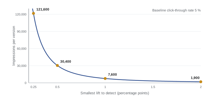
Statistical power is the probability that an experiment detects an effect of a given size if it truly exists. Underpowered experiments are common for creators: they run too briefly, conclude nothing has an effect, and abandon good ideas. Before running a test, estimate how much data you need. A widely used approximation for about 80 % power at the 5 % significance level gives the sample size per group as roughly 16 times the variance divided by the square of the smallest effect worth detecting.

Multiple comparisons

Each significance test at the 5 % level has a 5 % chance of a false positive, a result that looks significant by luck. If you test many metrics, segments or versions, false positives accumulate. With 10 independent tests and no real effects, the chance of at least one false positive is 1 − 0.95¹⁰ ≈ 40 %. Creators commonly fall into this trap by slicing results many ways, by country, device, traffic source and age group, and reporting whichever slice looks best. Remedies include choosing one primary metric in advance, treating other comparisons as exploratory, and, when several tests must be judged together, using a stricter threshold such as the Bonferroni correction, which divides 0.05 by the number of tests.

Peeking and stopping rules

Checking results repeatedly and stopping as soon as they look significant, called peeking, also inflates false positives, because random fluctuations cross the threshold at some point surprisingly often. Decide the sample size or duration in advance and judge the result then. Platforms' own testing tools manage this internally, which is one reason to prefer them when available.

A practical checklist

• Use medians or watch time rather than raw view averages when hits are skewed.
• Estimate the needed sample size before testing.
• Report effect sizes with confidence intervals, not just significance.
• Choose one primary metric and avoid slicing results many ways.
• Do not stop early because results look good; stick to the plan.
• Treat a single significant result as evidence, not proof, and confirm important findings with a repeat test.