Pretraining, transfer and scaling

Training a large network from scratch for every task wastes data and computation. The dominant pattern of modern deep learning is instead to pretrain one large model on a broad, plentiful source of data, often without labels, and then adapt it to many downstream tasks with little labelled data. This lesson covers transfer learning and fine-tuning, parameter-efficient adaptation methods such as LoRA, self-supervised and contrastive pretraining objectives, and the empirical scaling laws that relate a model's loss to its size, its data and its compute. It ends with a short introduction to graph neural networks, which extend the ideas of the course to data with irregular structure. AI-410 treats pretraining and adaptation of large language models in depth; the focus here is on the principles that apply across domains.

Transfer learning

The features a network learns on one task are often useful for others. The early layers of an image classifier trained on ImageNet detect edges, textures and parts that matter for almost any visual task; a language model trained to predict the next word must learn syntax, word meanings and facts that matter for almost any language task. Transfer learning reuses such a pretrained network as the starting point for a new target task. Jason Yosinski and colleagues (2014) measured how transferable each layer's features are and found early layers general and late layers increasingly specific to the source task.

There are two basic ways to transfer. A linear probe, or feature extraction, freezes the pretrained network, uses its last hidden layer as a fixed representation, and trains only a new output layer; it is cheap, cannot overfit much, and measures the quality of the representation. Fine-tuning initializes from the pretrained weights and continues training all or most of them on the target data, usually with a learning rate ten to a hundred times smaller than for pretraining so as not to destroy what was learned. Fine-tuning usually wins when the target task differs enough from the source or has a few thousand examples or more; linear probing can be competitive or better when target data are very scarce or the distributions differ in ways that fine-tuning distorts (Ananya Kumar and colleagues, 2022). A common compromise freezes the early layers and fine-tunes the later ones.

# Transfer learning in miniature: features learned on a large source task help a small related target task.
import numpy as np
rng = np.random.default_rng(466)
d, H, k = 40, 64, 6
P = rng.normal(size=(d, k)) / np.sqrt(d)            # six hidden features shared by both tasks
ref = np.maximum(0, rng.normal(size=(5000, d)) @ P * 2)
def task(n, w, seed):
    r = np.random.default_rng(seed)
    X = r.normal(size=(n, d)); z = np.maximum(0, X @ P * 2)
    s = z @ w - np.median(ref @ w)                   # shift so classes are roughly balanced
    return X, (s + 0.1 * r.normal(size=n) > 0).astype(float).reshape(-1, 1)
w_src, w_tgt = rng.normal(size=k), rng.normal(size=k)   # different heads on the same features
Xs, ys = task(20000, w_src, 1)
Xt, yt = task(60, w_tgt, 2); Xv, yv = task(4000, w_tgt, 3)

def train(X, y, W1=None, freeze=False, steps=1500, lr=0.5, seed=0):
    r = np.random.default_rng(seed)
    W1 = r.normal(0, np.sqrt(2 / d), (d, H)) if W1 is None else W1.copy()
    w2 = np.zeros((H, 1)); b = 0.0                   # a fresh output layer for every task
    for _ in range(steps):
        idx = r.choice(len(X), min(256, len(X)), replace=False)
        h = np.maximum(0, X[idx] @ W1); p = 1 / (1 + np.exp(-(h @ w2 + b)))
        g = (p - y[idx]) / len(idx)
        if not freeze:
            W1 -= lr * X[idx].T @ ((g @ w2.T) * (h > 0))
        w2 -= lr * h.T @ g; b -= lr * g.sum()
    return W1, w2, b
def acc(W1, w2, b, X, y): return np.mean(((np.maximum(0, X @ W1) @ w2 + b) > 0) == (y > 0.5))

W_pre, w_s, b_s = train(Xs, ys, steps=3000)                # "pretraining" on 20,000 source examples
print(f"source task accuracy after pretraining: {acc(W_pre, w_s, b_s, *task(3000, w_src, 9)):.3f}")
for name, kw in [("from scratch", {}), ("pretrained, frozen features (linear probe)", {"W1": W_pre, "freeze": True}),
                 ("pretrained, fine-tuned", {"W1": W_pre, "lr": 0.1})]:
    print(f"{name:42} target accuracy with 60 labels: {acc(*train(Xt, yt, **kw), Xv, yv):.3f}")

source task accuracy after pretraining: 0.965
from scratch                               target accuracy with 60 labels: 0.678
pretrained, frozen features (linear probe) target accuracy with 60 labels: 0.700
pretrained, fine-tuned                     target accuracy with 60 labels: 0.744

In the invented example both tasks depend on the same six hidden features of the input, combined differently. Trained from scratch, the target network must discover those features from 60 examples, and it reaches about 68 per cent accuracy. Pretraining on 20,000 source examples learns features that solve the source task at about 96 per cent. A linear probe on those frozen features does a little better than training from scratch, and fine-tuning them gently on the target data does better still, about 74 per cent, because the target task weights the shared features differently and benefits from adjusting them. The gains here are modest because the toy problem is small; with real pretrained models and scarce labels, the difference is often between a usable model and an unusable one. Real transfer works when, and to the extent that, the source and target share structure; transferring from an unrelated source can even hurt, which is called negative transfer.

Self-supervised pretraining

Labels are expensive; raw data are not. Self-supervised learning creates supervised tasks from unlabelled data by hiding part of each example and training the model to predict it. For text, the two main objectives are causal language modelling, predicting each token from the preceding ones (GPT), and masked language modelling, predicting randomly masked tokens from the rest (BERT, Jacob Devlin and colleagues, 2018). For images, masked autoencoders (Kaiming He and colleagues, 2022) hide most image patches and reconstruct them. Each objective forces the model to learn the structure of the data, and the resulting representations transfer to tasks the pretraining never mentioned.

Contrastive learning takes a different route: rather than reconstructing data, it learns an embedding in which related examples are close and unrelated ones are far apart. SimCLR (Ting Chen and colleagues, 2020) treats two random augmentations of the same image as a positive pair and other images in the batch as negatives. CLIP (Alec Radford and colleagues, 2021) trained on about 400 million image-caption pairs collected from the web, pulling each image's embedding toward its caption's and away from the other captions in the batch; the resulting model classifies images into categories it was never explicitly trained on, by comparing the image with text such as a photo of a dog. Both use the InfoNCE loss, a softmax cross-entropy over similarities in which the correct partner is the target class.

# The InfoNCE (contrastive) loss for a batch of paired embeddings, as in CLIP.
import numpy as np
rng = np.random.default_rng(466)
B, d = 6, 16
img = rng.normal(size=(B, d))
txt = img + 0.6 * rng.normal(size=(B, d))          # matching pairs are similar
def normalize(z): return z / np.linalg.norm(z, axis=1, keepdims=True)
def info_nce(a, b, tau):
    logits = normalize(a) @ normalize(b).T / tau      # B x B cosine similarities; diagonal = positives
    logits -= logits.max(1, keepdims=True)
    logp = logits - np.log(np.exp(logits).sum(1, keepdims=True))
    return -np.mean(np.diag(logp))
for tau in (1.0, 0.1, 0.07):
    print(f"temperature {tau:4}: loss with true pairs {info_nce(img, txt, tau):.3f}, "
          f"with shuffled pairs {info_nce(img, txt[rng.permutation(B)], tau):.3f}, chance level log B = {np.log(B):.3f}")

temperature  1.0: loss with true pairs 1.140, with shuffled pairs 1.971, chance level log B = 1.792
temperature  0.1: loss with true pairs 0.005, with shuffled pairs 4.987, chance level log B = 1.792
temperature 0.07: loss with true pairs 0.001, with shuffled pairs 12.433, chance level log B = 1.792

The temperature \(\tau\) controls how sharply the loss focuses on the hardest negatives. Lower temperatures make the true-pair loss smaller here, because the true partners are already the most similar, and make the loss for shuffled pairs larger. CLIP learns the temperature as a parameter. Contrastive methods need many negatives to work well, which is why they favour very large batches; methods such as BYOL and DINO avoid explicit negatives by predicting one view's embedding from another's with architectural asymmetries that prevent collapse to a constant.

Parameter-efficient fine-tuning

Fine-tuning every weight of a model with billions of parameters needs memory for gradients and optimizer state for all of them and produces a full copy of the model for every task. Parameter-efficient fine-tuning updates only a small number of parameters. Adapters (Neil Houlsby and colleagues, 2019) insert small bottleneck layers into each block and train only those. Prompt and prefix tuning learn a few continuous vectors prepended to the input or to each layer's keys and values. The most widely used method, LoRA (low-rank adaptation; Edward Hu and colleagues, 2021), freezes each pretrained weight matrix \(W_0\) and learns a low-rank update,

with B initialized to zero so that training starts exactly at the pretrained model. With rank 8 on a 1,024 × 1,024 matrix, LoRA trains 16,384 parameters instead of about a million. The update can be merged into \(W_0\) after training, so inference costs nothing extra, and many task-specific LoRA modules can share one base model. QLoRA (Tim Dettmers and colleagues, 2023) combines LoRA with a base model quantized to 4 bits, which brought fine-tuning of models with tens of billions of parameters within reach of a single GPU. LoRA works because fine-tuning updates appear to have low intrinsic dimension (Armen Aghajanyan and colleagues, 2021): the change needed to adapt a pretrained model lies close to a low-dimensional subspace.

# LoRA: the weight update for a 1,024 x 1,024 layer is restricted to B @ A with rank r.
import numpy as np
rng = np.random.default_rng(466)
d = 1024
for r in (4, 8, 16, 64):
    print(f"rank {r:2}: trainable {2 * d * r:7,} vs full {d * d:,} ({2 * d * r / (d * d):.2%})")
# If a full fine-tuning update happens to be approximately low rank, a small r captures most of it.
U = rng.normal(size=(d, 8)); Vt = rng.normal(size=(8, d))
delta = U @ Vt / 50 + rng.normal(0, 0.01, (d, d))        # rank-8 signal plus small full-rank noise
u, s, vt = np.linalg.svd(delta)
for r in (2, 8, 32):
    approx = (u[:, :r] * s[:r]) @ vt[:r]
    print(f"best rank-{r:2} approximation keeps {1 - np.linalg.norm(delta - approx) ** 2 / np.linalg.norm(delta) ** 2:.1%} of the update's energy")

rank  4: trainable   8,192 vs full 1,048,576 (0.78%)
rank  8: trainable  16,384 vs full 1,048,576 (1.56%)
rank 16: trainable  32,768 vs full 1,048,576 (3.12%)
rank 64: trainable 131,072 vs full 1,048,576 (12.50%)
best rank- 2 approximation keeps 29.1% of the update's energy
best rank- 8 approximation keeps 97.0% of the update's energy
best rank-32 approximation keeps 97.3% of the update's energy

Scaling laws

A striking empirical finding of the past decade is that a language model's test loss falls as a smooth power law in model size, data size and training compute, over many orders of magnitude. Joel Hestness and colleagues at Baidu (2017) observed power laws across several domains; Jared Kaplan and colleagues at OpenAI (2020) measured them carefully for transformers, finding that loss scales as \(L(N) \approx (N_c/N)^{\alpha_N}\) with \(\alpha_N\) around 0.076 for non-embedding parameters N, with similar laws in dataset size and compute, and that architectural details such as depth versus width matter much less than total scale. With the training compute rule \(C \approx 6ND\) for N parameters and D training tokens (lesson 8), the laws say how to divide a fixed compute budget between a bigger model and more data.

Kaplan and colleagues concluded that model size should grow much faster than data. Jordan Hoffmann and colleagues at DeepMind (2022) revisited the question with learning rate schedules matched to each run's length and found instead that parameters and tokens should grow in roughly equal proportion, about 20 tokens per parameter at the compute-optimal point. Their 70-billion-parameter Chinchilla, trained on 1.4 trillion tokens, outperformed their 280-billion-parameter Gopher, trained on 300 billion tokens with similar compute. Practice has since moved past compute-optimal training in one respect: because a smaller model is cheaper to run, models meant for wide deployment are often trained on far more than 20 tokens per parameter (the Llama 3 models of 2024 used more than 15 trillion tokens), accepting extra training compute to reduce inference cost.

# Fitting a power law L(C) = a * C**(-alpha) + L_inf to (invented) losses of models trained at increasing compute.
import numpy as np
rng = np.random.default_rng(466)
C = np.logspace(17, 21, 9)                       # training compute in FLOPs
L_true = 1.7 + 2.0e3 * C ** -0.16                # an assumed law, for illustration only
L = L_true * np.exp(rng.normal(0, 0.01, len(C)))
best = None
for L_inf in np.linspace(1.0, 2.0, 201):         # grid over the irreducible loss, linear fit in log space
    y = np.log(L - L_inf); X = np.c_[np.ones_like(C), np.log(C)]
    coef, res, *_ = np.linalg.lstsq(X, y, rcond=None)
    sse = np.sum((X @ coef - y) ** 2)
    if best is None or sse < best[0]:
        best = (sse, L_inf, coef)
_, L_inf, (loga, slope) = best
print(f"fitted: L_inf = {L_inf:.3f}, alpha = {-slope:.3f}, a = {np.exp(loga):.3g}   (true 1.700, 0.160, 2.00e+03)")
for c in (1e22, 1e23):
    print(f"extrapolated loss at C = {c:.0e}: {L_inf + np.exp(loga) * c ** slope:.3f}")

fitted: L_inf = 1.580, alpha = 0.151, a = 1.43e+03   (true 1.700, 0.160, 2.00e+03)
extrapolated loss at C = 1e+22: 2.273
extrapolated loss at C = 1e+23: 2.070

# Compute-optimal allocation in the Chinchilla style: with C = 6 N D and D about 20 N, solve for N and D.
for C in (1e21, 1e23, 1e25):
    N = (C / (6 * 20)) ** 0.5            # parameters
    D = 20 * N                           # training tokens
    print(f"C = {C:.0e} FLOPs: about {N / 1e9:7.2f} billion parameters trained on {D / 1e9:8.1f} billion tokens")
# Gopher (280 B parameters, 300 B tokens) versus Chinchilla (70 B, 1.4 T) used similar compute:
for name, N, D in (("Gopher", 280e9, 300e9), ("Chinchilla", 70e9, 1.4e12)):
    print(f"{name:10}: C = 6ND = {6 * N * D:.2e} FLOPs, tokens per parameter {D / N:.1f}")

C = 1e+21 FLOPs: about    2.89 billion parameters trained on     57.7 billion tokens
C = 1e+23 FLOPs: about   28.87 billion parameters trained on    577.4 billion tokens
C = 1e+25 FLOPs: about  288.68 billion parameters trained on   5773.5 billion tokens
Gopher    : C = 6ND = 5.04e+23 FLOPs, tokens per parameter 1.1
Chinchilla: C = 6ND = 5.88e+23 FLOPs, tokens per parameter 20.0

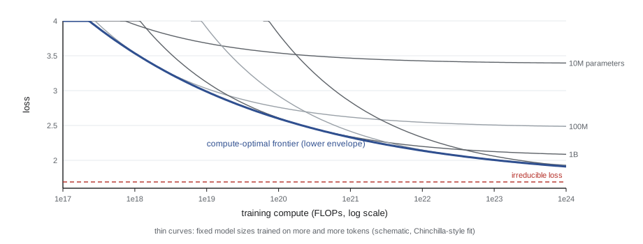
Scaling laws must be used with care. They describe the loss on the training distribution, not any particular capability; some capabilities appear to emerge abruptly with scale, although Rylan Schaeffer and colleagues (2023) argued that much of the apparent abruptness comes from discontinuous evaluation metrics. They depend on the data: repeated data gives diminishing returns (Niklas Muennighoff and colleagues, 2023), and the supply of high-quality text is finite, a constraint widely discussed as of 2026. And extrapolating any fit far beyond the measured range is risky, as the invented example shows: with just 1 per cent noise on nine points, the fitted irreducible loss comes out at 1.58 instead of the true 1.70, and the exponent at 0.151 instead of 0.160, so its extrapolations are biased low, by an amount that grows with the distance of the extrapolation. Still, scaling laws turned the planning of large training runs from guesswork into engineering, by letting labs fit the laws on small runs and predict the result of a large one.

Foundation models and in-context learning

Models pretrained at scale and adapted to many tasks are often called foundation models (Rishi Bommasani and colleagues, 2021). Large language models showed a further form of transfer: in-context learning, in which the model performs a new task given only instructions and a few examples in its input, with no weight updates at all (Tom Brown and colleagues, GPT-3, 2020). Instruction tuning and reinforcement learning from human feedback then align a pretrained model's behaviour with what users want. AI-410 covers these methods, and AI-430 the safety questions they raise.

Graph neural networks

Not all data lie on grids or sequences. Molecules, social networks, road maps and knowledge bases are graphs, and graph neural networks (GNNs) extend the idea of a shared local operation to them. In a message-passing layer, each node gathers messages from its neighbours, aggregates them with an operation that does not depend on their order (sum, mean or max), and updates its own representation. The graph convolutional network of Thomas Kipf and Max Welling (2017) uses \(H' = \sigma(\hat{D}^{-1/2}\hat{A}\hat{D}^{-1/2}HW)\), where \(\hat{A}\) is the adjacency matrix with self-loops and \(\hat{D}\) its degree matrix. Because the operation treats all nodes alike and aggregates neighbours symmetrically, relabelling the nodes just relabels the outputs, the graph analogue of translation equivariance. Graph attention networks weight neighbours by learned attention, and transformers can be seen as GNNs on a fully connected graph. GNNs are central to molecular property prediction and drug discovery, recommendation systems and traffic forecasting; DeepMind's GraphCast (2023) uses one for medium-range weather forecasting.

# One round of graph message passing (a simplified graph convolution) on a 5-node graph.
import numpy as np
A = np.array([[0, 1, 1, 0, 0], [1, 0, 1, 0, 0], [1, 1, 0, 1, 0], [0, 0, 1, 0, 1], [0, 0, 0, 1, 0]], dtype=float)
X = np.array([[1, 0], [1, 0], [0, 1], [0, 1], [0, 1]], dtype=float)   # two input features per node
Ah = A + np.eye(5)                                   # include each node's own features
Dinv = np.diag(1 / np.sqrt(Ah.sum(1)))
S = Dinv @ Ah @ Dinv                                 # symmetric normalization (Kipf and Welling, 2017)
W = np.array([[1.0, -0.5], [0.5, 1.0]])
H = np.maximum(0, S @ X @ W)
print("node features after one layer (each node mixes in the nodes it is linked to):")
print(np.round(H, 3))
perm = np.array([4, 2, 0, 1, 3]); Pm = np.eye(5)[perm]
H2 = np.maximum(0, (Pm @ S @ Pm.T) @ (Pm @ X) @ W)
print("relabelling the nodes just relabels the output:", np.allclose(H2, Pm @ H))

node features after one layer (each node mixes in the nodes it is linked to):
[[0.811 0.   ]
 [0.811 0.   ]
 [0.847 0.25 ]
 [0.515 1.03 ]
 [0.454 0.908]]
relabelling the nodes just relabels the output: True

Worked examples