Optimization for deep learning

With gradients in hand, training is an optimization problem: minimize the average training loss \(\mathcal{L}(\theta) = \frac{1}{N}\sum_i \ell(f_\theta(\mathbf{x}_i), y_i)\) over millions or billions of parameters. The problem is non-convex, the data are too large to touch in full at every step, and the quantity that actually matters, error on new data, is not the one being minimized. This lesson covers the optimizers used to train deep networks in practice: stochastic gradient descent and its momentum variants, the adaptive methods RMSProp, Adam and AdamW, learning rate schedules with warmup, the effect of batch size, and what is known about the loss landscapes these methods navigate. AI-310 develops the convergence theory of these methods in depth; here the emphasis is on behaviour, practical choices and the reasons behind them.

Stochastic gradient descent

Gradient descent updates \(\theta \gets \theta - \eta \nabla \mathcal{L}(\theta)\), where \(\eta\) is the learning rate. Computing the full gradient needs a pass over all N examples, which is wasteful when N is in the millions and neighbouring examples carry similar information. Stochastic gradient descent (SGD) instead estimates the gradient from a random mini-batch of B examples, \(\mathbf{g} = \frac{1}{B}\sum_{i \in \mathcal{B}} \nabla \ell_i\), which is an unbiased estimate of the full gradient whose variance falls like 1/B. An epoch is one pass through the training set in mini-batches, usually after shuffling.

The noise in SGD is not only a cost. Many updates per epoch make early progress fast, and the noise helps the iterates escape saddle points and sharp regions of the landscape. The learning rate controls a balance between progress and noise: too large and training diverges or oscillates, too small and it crawls. On a quadratic with largest curvature \(\lambda_{\max}\) (the largest eigenvalue of the Hessian), plain gradient descent converges only if \(\eta < 2/\lambda_{\max}\), and its speed along the flattest direction is governed by \(\eta\lambda_{\min}\). The ratio \(\kappa = \lambda_{\max}/\lambda_{\min}\), the condition number, therefore sets how slow gradient descent must be: the step is capped by the steepest direction and progress is limited by the flattest.

Momentum and Nesterov momentum

Momentum, due to Boris Polyak (1964), keeps a running velocity \(\mathbf{v} \gets \beta\mathbf{v} + \mathbf{g}\) and steps along it, \(\theta \gets \theta - \eta\mathbf{v}\), with \(\beta\) typically 0.9. In a long narrow valley the gradient components across the valley alternate in sign and cancel in the velocity, while the components along the valley floor point consistently and accumulate. The effective step along consistent directions grows by up to a factor \(1/(1 - \beta)\), ten times for \(\beta = 0.9\). Nesterov's accelerated gradient (Yurii Nesterov, 1983) evaluates the gradient at the point the momentum is about to carry the parameters to, which corrects overshooting earlier; Ilya Sutskever, James Martens, George Dahl and Geoffrey Hinton (2013) showed that SGD with Nesterov momentum and a good schedule trains deep networks well. For convex quadratics, heavy-ball momentum improves the dependence on the condition number from \(\kappa\) to \(\sqrt{\kappa}\).

Adaptive methods: AdaGrad, RMSProp and Adam

Different parameters often need different step sizes: embeddings of rare words get few gradient signals, while biases of busy units get many. AdaGrad (John Duchi, Elad Hazan and Yoram Singer, 2011) divides each coordinate's step by the square root of the sum of its past squared gradients, so frequently updated coordinates slow down. Its accumulated sum only grows, so its steps eventually become too small for long non-convex training. RMSProp, proposed by Geoffrey Hinton in a 2012 course lecture, replaces the sum with an exponential moving average \(r \gets \rho r + (1 - \rho)g^2\), so the scale adapts to recent gradients.

Adam (Diederik Kingma and Jimmy Ba, 2015) combines momentum with RMSProp's scaling. It keeps moving averages of the gradient and of its square,

where \(\hat{\mathbf{m}} = \mathbf{m}/(1 - \beta_1^t)\) and \(\hat{\mathbf{v}} = \mathbf{v}/(1 - \beta_2^t)\) correct the bias toward zero of averages started at zero, and the defaults \(\beta_1 = 0.9\), \(\beta_2 = 0.999\), \(\epsilon = 10^{-8}\) work across a wide range of problems. Because the update divides the gradient by its own typical magnitude, each coordinate moves by roughly \(\eta\) per step regardless of the gradient's scale, which makes Adam far less sensitive to the scaling of parameters and losses than SGD. It is the default optimizer for transformers and most large models.

# Five optimizers on an ill-conditioned valley: f(x, y) = 0.5 * (x**2 + 50 * y**2), started at (-8, 1).
import numpy as np
grad = lambda p: np.array([p[0], 50 * p[1]])
f = lambda p: 0.5 * (p[0] ** 2 + 50 * p[1] ** 2)
def run(step, n=100):
    p = np.array([-8.0, 1.0]); state = {}
    for t in range(1, n + 1):
        p = step(p, grad(p), state, t)
    return p
def sgd(lr):
    return lambda p, g, s, t: p - lr * g
def momentum(lr, beta=0.9):
    def step(p, g, s, t):
        s["v"] = beta * s.get("v", 0) + g            # velocity accumulates past gradients
        return p - lr * s["v"]
    return step
def nesterov(lr, beta=0.9):
    def step(p, g, s, t):
        v_old = s.get("v", 0); s["v"] = beta * v_old + g
        return p - lr * (g + beta * s["v"])         # look-ahead form used by most libraries
    return step
def rmsprop(lr, rho=0.99, eps=1e-8):
    def step(p, g, s, t):
        s["r"] = rho * s.get("r", 0) + (1 - rho) * g ** 2
        return p - lr * g / (np.sqrt(s["r"]) + eps)  # per-coordinate step size
    return step
def adam(lr, b1=0.9, b2=0.999, eps=1e-8):
    def step(p, g, s, t):
        s["m"] = b1 * s.get("m", 0) + (1 - b1) * g
        s["v"] = b2 * s.get("v", 0) + (1 - b2) * g ** 2
        mh = s["m"] / (1 - b1 ** t); vh = s["v"] / (1 - b2 ** t)   # bias correction
        return p - lr * mh / (np.sqrt(vh) + eps)
    return step
print("largest stable plain-GD step: 2 / 50 =", 2 / 50)
for name, opt in [("GD, lr 0.039", sgd(0.039)), ("GD, lr 0.041", sgd(0.041)), ("momentum, lr 0.02", momentum(0.02)),
                  ("Nesterov, lr 0.02", nesterov(0.02)), ("RMSProp, lr 0.1", rmsprop(0.1)), ("Adam, lr 0.5", adam(0.5))]:
    p = run(opt)
    print(f"{name:18} after 100 steps: f = {f(p):10.3e}   point ({p[0] + 0.0:8.4f}, {round(p[1], 4) + 0.0:8.4f})")

largest stable plain-GD step: 2 / 50 = 0.04
GD, lr 0.039       after 100 steps: f =  1.209e-02   point ( -0.1498,   0.0059)
GD, lr 0.041       after 100 steps: f =  4.323e+05   point ( -0.1216, 131.5013)
momentum, lr 0.02  after 100 steps: f =  6.176e-04   point ( -0.0338,   0.0014)
Nesterov, lr 0.02  after 100 steps: f =  1.041e-04   point ( -0.0144,   0.0000)
RMSProp, lr 0.1    after 100 steps: f =  7.112e-05   point ( -0.0119,   0.0000)
Adam, lr 0.5       after 100 steps: f =  1.305e-03   point ( -0.0408,  -0.0043)

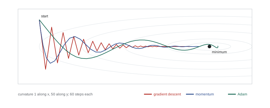
The output illustrates the condition number at work. The valley has curvatures 1 and 50, so plain gradient descent must keep its learning rate below 2/50 = 0.04; at 0.041 it diverges along the steep axis. Even at 0.039 it makes slow progress along the flat axis, because \(0.039 \times 1\) is small. Momentum and Nesterov reach far lower losses in the same 100 steps. RMSProp and Adam rescale the two coordinates to similar effective step sizes and so are nearly insensitive to the conditioning, although at a fixed learning rate they hover around the minimum at a distance set by the step size rather than converging exactly; that is one reason schedules decay the learning rate.

AdamW and weight decay

Weight decay shrinks weights toward zero at every step, \(\theta \gets \theta - \eta\lambda\theta\). For plain SGD this is the same as adding an L2 penalty \(\frac{\lambda}{2}\lVert\theta\rVert^2\) to the loss. For Adam it is not: an L2 penalty adds \(\lambda\theta\) to the gradient, which then gets divided by \(\sqrt{\hat{v}}\), so parameters with large gradients are barely regularized and parameters with small gradients are regularized heavily. Ilya Loshchilov and Frank Hutter (2019) proposed AdamW, which applies the decay directly to the weights, decoupled from the adaptive scaling, and showed that it generalizes better. AdamW, with decay around 0.01 to 0.1 and typically not applied to biases and normalization parameters, is the standard optimizer for transformer training.

# L2 penalty in the loss versus decoupled weight decay (AdamW): with Adam they are not the same.
import numpy as np
rng = np.random.default_rng(466)
X = rng.normal(size=(200, 5)) * np.array([1, 1, 1, 10, 0.1])   # features on very different scales
y = X @ np.array([1.0, -2.0, 0.5, 0.3, 4.0]) + rng.normal(0, 0.5, 200)
def train(decoupled, lam=0.1, lr=0.01, steps=3000):
    w = np.zeros(5); m = np.zeros(5); v = np.zeros(5)
    for t in range(1, steps + 1):
        g = X.T @ (X @ w - y) / len(X)
        if not decoupled:
            g = g + lam * w                             # L2 penalty enters the adaptive scaling
        m = 0.9 * m + 0.1 * g; v = 0.999 * v + 0.001 * g ** 2
        step = (m / (1 - 0.9 ** t)) / (np.sqrt(v / (1 - 0.999 ** t)) + 1e-8)
        w = w - lr * step
        if decoupled:
            w = w - lr * lam * w                        # decay applied directly to the weights
    return w
print("Adam + L2 penalty:", np.round(train(False), 3))
print("AdamW (decoupled):", np.round(train(True), 3))
print("least squares     :", np.round(np.linalg.lstsq(X, y, rcond=None)[0], 3))

Adam + L2 penalty: [ 0.848 -1.817  0.443  0.295  0.328]
AdamW (decoupled): [ 0.928 -1.968  0.502  0.298  3.747]
least squares     : [ 0.933 -1.994  0.504  0.298  3.988]

The fifth feature has a tiny scale, so its true coefficient of 4 produces small gradients. Under Adam with an L2 penalty, the penalty term dominates that coordinate's gradient, and the adaptive scaling turns it into a full-size step toward zero: the coefficient collapses to about 0.3. Under AdamW the decay shrinks each weight by the same small fraction per step, so the fifth coefficient stays near its least-squares value, as do the others. Regularization strength that depends on a feature's units, rather than on how much the coefficient matters, is rarely what anyone wants.

Learning rate schedules and warmup

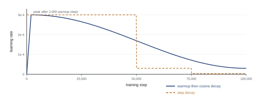
A constant learning rate is rarely best. Early in training, large steps make fast progress; late in training, the noise of large steps keeps the parameters bouncing around a minimum, and smaller steps let them settle. Common schedules are step decay (divide by 10 at fixed epochs, standard for ResNets), cosine decay (Loshchilov and Hutter, 2017), which follows half a cosine curve from the peak rate to a small floor, and the inverse square root schedule of the original transformer. The one-cycle policy of Leslie Smith raises the rate and then lowers it within a single run.

Warmup starts with a small learning rate and increases it linearly over the first few hundred or thousand steps. It matters most for Adam and for transformers. At the start of training, Adam's second-moment estimate is based on very few gradients and can be unreliably small, producing very large steps; the network's activations and gradients are also far from their typical scales. A short warmup lets these settle before full-size steps begin. Without warmup, transformer training often diverges in the first few hundred steps. Linear warmup to a peak followed by cosine decay is the most common schedule for large models.

# Linear warmup followed by cosine decay, the most common schedule for training transformers.
import math
peak, warm, total, floor = 3e-4, 2000, 100000, 3e-5
def lr(step):
    if step < warm:
        return peak * (step + 1) / warm
    progress = (step - warm) / (total - warm)
    return floor + 0.5 * (peak - floor) * (1 + math.cos(math.pi * progress))
for s in (0, 500, 1999, 2000, 25000, 50000, 75000, 99999):
    print(f"step {s:6}: learning rate {lr(s):.2e}")

step      0: learning rate 1.50e-07
step    500: learning rate 7.51e-05
step   1999: learning rate 3.00e-04
step   2000: learning rate 3.00e-04
step  25000: learning rate 2.65e-04
step  50000: learning rate 1.69e-04
step  75000: learning rate 7.11e-05
step  99999: learning rate 3.00e-05

Batch size

The batch size trades statistical efficiency against hardware efficiency. Gradient noise shrinks like \(1/\sqrt{B}\), as the next program confirms, so larger batches give more accurate steps; but each step costs B examples, and beyond some point doubling B no longer halves the number of steps needed. Sam McCandlish and colleagues at OpenAI (2018) called this point the critical batch size and showed that it can be estimated from the gradient noise scale; it tends to grow as training progresses and the loss falls. Below it, larger batches are nearly free speedups on parallel hardware; above it, they waste computation.

# Mini-batch gradient noise: the spread of a gradient estimate shrinks like 1/sqrt(batch size).
import numpy as np
rng = np.random.default_rng(466)
N = 20000
X = rng.normal(size=(N, 10)); w_true = rng.normal(size=10)
y = X @ w_true + rng.normal(0, 1.0, N)
w = np.zeros(10)                                       # evaluate gradients at a fixed point
full = X.T @ (X @ w - y) / N                           # the full-batch gradient of mean squared error / 2
for B in (8, 32, 128, 512, 2048):
    errs = []
    for _ in range(300):
        idx = rng.choice(N, B, replace=False)
        g = X[idx].T @ (X[idx] @ w - y[idx]) / B
        errs.append(np.linalg.norm(g - full))
    print(f"batch {B:5}: mean distance from full gradient {np.mean(errs):6.3f}   x sqrt(B) = {np.mean(errs) * np.sqrt(B):5.2f}")

batch     8: mean distance from full gradient  2.337   x sqrt(B) =  6.61
batch    32: mean distance from full gradient  1.258   x sqrt(B) =  7.12
batch   128: mean distance from full gradient  0.621   x sqrt(B) =  7.02
batch   512: mean distance from full gradient  0.303   x sqrt(B) =  6.85
batch  2048: mean distance from full gradient  0.142   x sqrt(B) =  6.42

When the batch size changes, the learning rate should usually change with it. For SGD, Priya Goyal and colleagues at Facebook (2017) trained ResNet-50 on ImageNet in one hour with batches of 8,192 by scaling the learning rate linearly with the batch size and using warmup; for Adam, a square root rule is often closer. Very large batches can also hurt generalization, an effect attributed by Nitish Keskar and colleagues (2017) to convergence to sharper minima, although later work showed much of the gap can be closed by retuning the learning rate and schedule.

The loss landscape

Deep network losses are non-convex, yet gradient methods train them reliably. Several findings explain why this is less alarming than it sounds. In high dimensions, most critical points are saddle points rather than poor local minima (Yann Dauphin and colleagues, 2014), and noisy gradient methods escape saddles. Many minima are equivalent: permuting the hidden units of a layer gives the same function with different weights, so minima come in large symmetric families. In overparameterized networks, minima found from different initializations are often connected by paths of low loss (Timur Garipov and colleagues; Felix Draxler and colleagues, both 2018). And the minima reached tend to generalize well, although why remains an active research question that lesson 5 returns to.

Training dynamics also show regularities. Jeremy Cohen and colleagues (2021) observed that full-batch gradient descent drives the sharpness (the top Hessian eigenvalue) up until it hovers near \(2/\eta\), the edge of stability, while the loss keeps decreasing non-monotonically. Practical consequences are the familiar heuristics: if the loss spikes or diverges, lower the learning rate or lengthen warmup; if it plateaus early, raise it. A learning rate range test, which increases the rate exponentially over a few hundred steps and plots the loss, finds a usable range quickly.

Gradient clipping and second-order ideas

Occasional huge gradients, from an unlucky batch or a sharp cliff in the landscape, can undo much of training in one step. Gradient clipping rescales the whole gradient vector whenever its norm exceeds a threshold c, \(\mathbf{g} \gets \mathbf{g} \cdot \min(1, c/\lVert\mathbf{g}\rVert)\). It was introduced for recurrent networks (Razvan Pascanu, Tomas Mikolov and Yoshua Bengio, 2013) and is now routine in transformer training with c around 1.0.

Second-order methods use curvature to choose better steps. Newton's method is impractical for millions of parameters, because the Hessian has a trillion entries for a million parameters, but approximations exist: K-FAC approximates curvature layer by layer with Kronecker products, Shampoo uses preconditioners for each weight matrix's rows and columns, and recent methods such as Muon orthogonalize the update matrix for each layer. Some of these have shown speedups over AdamW in published comparisons, but AdamW remains the default in most large-scale training as of 2026. AI-310 covers these methods and their theory.

Worked examples