From linear models to deep networks

Deep learning is the study of models built by composing many simple, differentiable functions, called layers, and fitting all of their parameters together by gradient descent on a loss. CMPUT-367 ended with a two-layer network that learned exclusive or by backpropagation. This course starts from that point and builds up the ideas that make networks with dozens or hundreds of layers and billions of parameters trainable: automatic differentiation, adaptive optimizers, careful initialization and normalization, residual connections, regularization, and the architectures (convolutional, recurrent and attention-based) that build knowledge about the structure of data into the network. Throughout, the course implements each idea from scratch in NumPy on small, invented and seeded data, so that every number in the stored outputs can be reproduced and every gradient can be checked.

This lesson sets up the vocabulary. It describes a feedforward network as a composition of affine maps and nonlinearities, compares the common activation functions, states what the universal approximation theorem does and does not promise, and explains why depth, rather than width alone, is what made deep learning work. It ends by training a small network on a problem no linear model can solve.

Why go beyond linear models

A linear model scores an input \(\mathbf{x} \in \mathbb{R}^d\) as \(\mathbf{w}^{\top}\mathbf{x} + b\). Logistic regression, linear regression and linear support vector machines all share this form and differ only in the loss. They are convex to fit, well understood and often hard to beat on small tabular problems, as the CMPUT-367 capstone showed. Their weakness is representational: the decision boundary is a hyperplane in the input space. CMPUT-367 offered two ways around that. Feature engineering builds nonlinear features by hand (polynomials, interactions, binned values), and kernel methods build them implicitly through a kernel function. Both fix the features before learning begins.

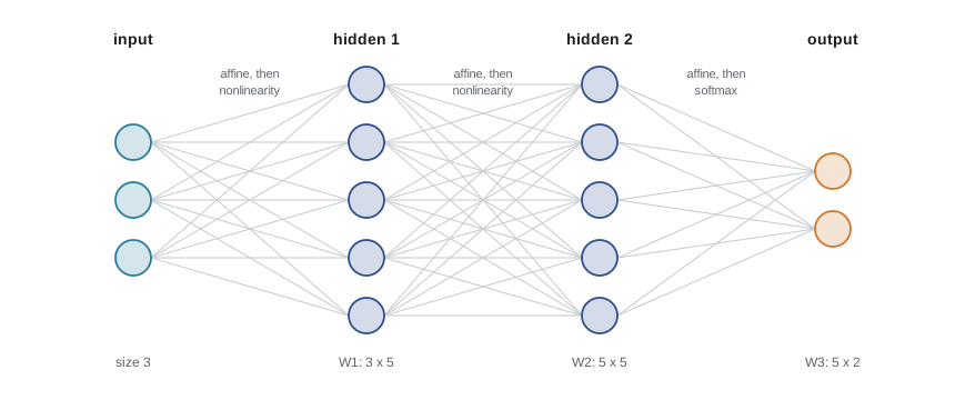
Neural networks learn the features. A hidden layer computes \(\mathbf{h} = \phi(W\mathbf{x} + \mathbf{b})\), where W is a weight matrix, \(\mathbf{b}\) a bias vector and \(\phi\) a nonlinear function applied elementwise. The next layer treats \(\mathbf{h}\) as its input. Because W is learned, the network chooses its own features to suit the task, and because layers can be stacked, it can build features of features. For images, early layers come to detect edges, middle layers textures and parts, and late layers whole objects; for text, layers progress from characters and word pieces to syntax and meaning. This learned hierarchy of representations is the central idea of deep learning, and the reason the field is also called representation learning.

The feedforward network

A feedforward network, or multilayer perceptron (MLP), with L layers computes

where g is the output function chosen to match the task: the identity for regression, the logistic sigmoid for binary classification, the softmax for several classes. The parameters \(\theta = \{W^{(\ell)}, \mathbf{b}^{(\ell)}\}\) are fitted by minimizing an average loss over the training set, exactly as in empirical risk minimization. The pre-activation \(\mathbf{z}^{(\ell)} = W^{(\ell)}\mathbf{h}^{(\ell-1)} + \mathbf{b}^{(\ell)}\) and the activation \(\mathbf{h}^{(\ell)} = \phi(\mathbf{z}^{(\ell)})\) are worth naming separately, because backpropagation in lesson 2 needs both.

Without the nonlinearity \(\phi\) the whole stack collapses: a product of matrices is a matrix, so an L-layer linear network computes the same functions as one linear layer. Its training problem is different (non-convex, with interesting dynamics that theorists study), but its expressive power is no greater. The nonlinearity is what makes depth meaningful.

In code, data are processed in mini-batches. With a batch of B examples stored as the rows of a matrix X of shape \(B \times d\), a layer is computed as \(H = \phi(XW + \mathbf{b})\) with W of shape \(d \times k\) and the bias broadcast across rows. This row convention, used by NumPy, PyTorch and JAX, is the one used in all code in this course; the equations use the column convention of most textbooks. Shapes are the first thing to check when a network misbehaves.

Activation functions

The choice of \(\phi\) matters more for training than for expressive power, because it controls how gradients flow. The classic choices were the logistic sigmoid \(\sigma(z) = 1/(1 + e^{-z})\) and the hyperbolic tangent. Both saturate: for large \(|z|\) their slopes approach zero. The sigmoid's slope is at most 0.25, at \(z = 0\), so a gradient passing backward through ten sigmoid layers is multiplied by at most \(0.25^{10} \approx 10^{-6}\). This vanishing gradient problem, analysed by Sepp Hochreiter in his 1991 thesis, is one reason deep networks were hard to train before about 2010.

The rectified linear unit, \(\mathrm{ReLU}(z) = \max(0, z)\), popularized for deep networks by Vinod Nair and Geoffrey Hinton (2010) and Xavier Glorot, Antoine Bordes and Yoshua Bengio (2011), has slope exactly 1 for positive inputs, so it does not shrink gradients where it is active, and it is very cheap to compute. Its weakness is the dead unit: a unit whose pre-activation is negative for every input passes no gradient and never recovers. Variants address this. Leaky ReLU uses a small slope such as 0.01 for negative inputs. The exponential linear unit (ELU) is smooth at zero. The Gaussian error linear unit, \(\mathrm{GELU}(z) = z\,\Phi(z)\) with \(\Phi\) the standard normal cumulative distribution function (Dan Hendrycks and Kevin Gimpel, 2016), and the closely related SiLU or swish, \(z\,\sigma(z)\), are smooth curves that behave like ReLU for large \(|z|\) and dip slightly below zero near the origin. GELU is the default in BERT and GPT-style transformers; gated variants such as SwiGLU, which multiply one linear projection by the swish of another, are standard in recent large language models (AI-410 covers them).

# Activation functions and their derivatives at a few points, and what saturation does to gradients.
import numpy as np
z = np.array([-6.0, -2.0, -0.5, 0.0, 0.5, 2.0, 6.0])
sig = 1 / (1 + np.exp(-z))
acts = {
    "sigmoid": (sig, sig * (1 - sig)),
    "tanh":    (np.tanh(z), 1 - np.tanh(z) ** 2),
    "ReLU":    (np.maximum(0, z), (z > 0).astype(float)),
    "GELU":    (0.5 * z * (1 + np.tanh(np.sqrt(2 / np.pi) * (z + 0.044715 * z ** 3))), None),
}
# GELU derivative by a central difference (its closed form is long)
h = 1e-5
g = lambda t: 0.5 * t * (1 + np.tanh(np.sqrt(2 / np.pi) * (t + 0.044715 * t ** 3)))
acts["GELU"] = (acts["GELU"][0], (g(z + h) - g(z - h)) / (2 * h))
print("z        " + " ".join(f"{v:7.2f}" for v in z))
for name, (f, d) in acts.items():
    print(f"{name:8} " + " ".join(f"{round(float(v), 3) + 0.0:7.3f}" for v in f))
    print(f"  slope  " + " ".join(f"{round(float(v), 3) + 0.0:7.3f}" for v in d))
# a chain of 10 sigmoid layers multiplies at most ten slopes of 0.25
print("largest possible gradient factor through 10 sigmoids:", 0.25 ** 10)

z          -6.00   -2.00   -0.50    0.00    0.50    2.00    6.00
sigmoid    0.002   0.119   0.378   0.500   0.622   0.881   0.998
  slope    0.002   0.105   0.235   0.250   0.235   0.105   0.002
tanh      -1.000  -0.964  -0.462   0.000   0.462   0.964   1.000
  slope    0.000   0.071   0.786   1.000   0.786   0.071   0.000
ReLU       0.000   0.000   0.000   0.000   0.500   2.000   6.000
  slope    0.000   0.000   0.000   0.000   1.000   1.000   1.000
GELU       0.000  -0.045  -0.154   0.000   0.346   1.955   6.000
  slope    0.000  -0.086   0.133   0.500   0.867   1.086   1.000
largest possible gradient factor through 10 sigmoids: 9.5367431640625e-07

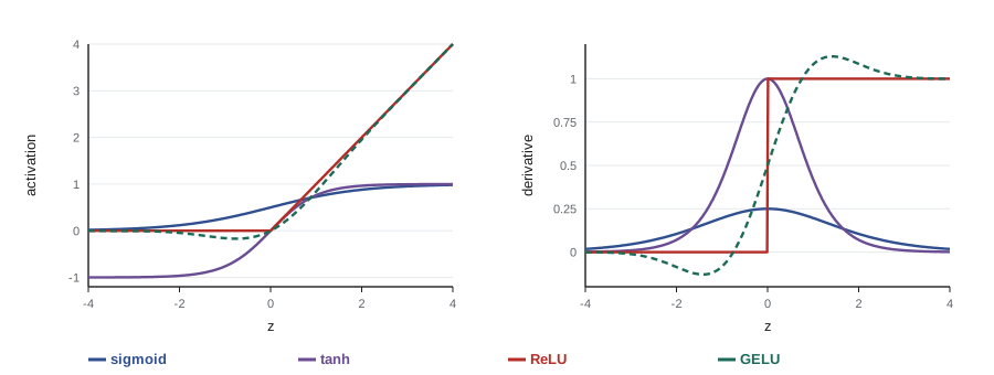
The output shows the pattern. At \(z = \pm 6\) the sigmoid and tanh slopes are essentially zero, while ReLU and GELU keep a slope of 1 on the positive side. That one property, more than anything else, explains why ReLU-family activations replaced sigmoids in hidden layers. Sigmoids survive where an output must lie in (0, 1): binary outputs, and the gates of the LSTM in lesson 7.

Universal approximation and its limits

How expressive is a network? The universal approximation theorem, proved for sigmoid units by George Cybenko (1989) and for general non-polynomial activations by Kurt Hornik, Maxwell Stinchcombe and Halbert White (1989) and Moshe Leshno and colleagues (1993), says that a network with a single hidden layer and enough units can approximate any continuous function on a compact set to any accuracy. The intuition for ReLU in one dimension is simple: a sum of shifted ReLUs is a piecewise linear function with a kink at each shift, and piecewise linear functions with enough pieces approximate any continuous curve.

The theorem is reassuring but says three things less than it seems to. It says nothing about how many units are needed, and for some functions the number grows exponentially with the input dimension. It says nothing about whether gradient descent will find the approximating weights. And it says nothing about generalization: a network that can fit any function can also fit noise, a point lesson 5 returns to with the experiment of Chiyuan Zhang and colleagues (2017), who trained standard image networks to perfect accuracy on randomly shuffled labels.

Why depth helps

If one hidden layer suffices in principle, why build deep networks? Because deep networks can represent some functions with exponentially fewer units than shallow ones. A clean example is due to Matus Telgarsky (2016). The tent map \(t(x) = 2x\) for \(x \le 1/2\) and \(2 - 2x\) for \(x > 1/2\) is computed on [0, 1] by a layer of two ReLU units. Composing it with itself k times produces a sawtooth with \(2^k\) linear pieces, using only 2k units. A single hidden layer with n ReLU units on a one-dimensional input produces at most n + 1 pieces, so matching the sawtooth needs about \(2^k\) units. Depth multiplies the number of pieces; width only adds to it.

# Depth versus width: how many linear regions can a ReLU network carve the line [0, 1] into?
# A one-hidden-layer net with n units has at most n + 1 pieces. Composing a "tent" map k times
# (two ReLU units per layer) gives 2**k pieces with only 2k units.
import numpy as np
x = np.linspace(0, 1, 200001)
def tent(t):                       # tent(t) = 2*relu(t) - 4*relu(t - 0.5), a 2-unit ReLU layer
    return 2 * np.maximum(0, t) - 4 * np.maximum(0, t - 0.5)
def pieces(y):                     # count linear pieces by counting slope changes
    s = np.sign(np.round(np.diff(y) / np.diff(x), 6))
    return 1 + int(np.sum(s[1:] != s[:-1]))
y = x.copy()
for k in range(1, 7):
    y = tent(y)
    print(f"depth {k}: {2 * k:2} hidden units, {pieces(y):3} linear pieces")
print("a single hidden layer with 12 units gives at most", 12 + 1, "pieces")

depth 1:  2 hidden units,   2 linear pieces
depth 2:  4 hidden units,   4 linear pieces
depth 3:  6 hidden units,   8 linear pieces
depth 4:  8 hidden units,  16 linear pieces
depth 5: 10 hidden units,  32 linear pieces
depth 6: 12 hidden units,  64 linear pieces
a single hidden layer with 12 units gives at most 13 pieces

Six layers of two units each, twelve units in all, carve the interval into 64 pieces, where twelve units in one layer manage at most 13. Real data are not sawtooths, but the same principle applies: compositional structure, in which complex features are built from simpler ones, is cheap to represent with depth. Images, speech and language are full of such structure. The practical evidence came between 2006 and 2016, when deeper networks steadily won on speech recognition and image classification, culminating in residual networks with more than a hundred layers (lesson 4).

Depth has costs. Deeper networks are harder to optimize, because gradients must pass through many layers and can vanish or explode; most of lessons 3 and 4 concern the techniques that tame this. They are also more sequential to compute, which matters for latency on hardware, the subject of AI-480.

A first deep network

The program below trains a network with two hidden layers of 32 ReLU units on the two-spirals problem, a classic test in which two interleaved spirals must be separated. It writes the forward pass, the loss and every gradient by hand, which lesson 2 will replace with automatic differentiation. Note two details that will recur. First, the loss is computed from the score s with \(\log(1 + e^{s}) - ys\), using NumPy's logaddexp, rather than by taking logarithms of probabilities: this is the same quantity as binary cross-entropy but never overflows or takes the logarithm of zero. Second, the gradient of that loss with respect to the score is simply \(p - y\), the same tidy form as in logistic regression.

# A two-hidden-layer network trained from scratch with NumPy on an invented two-spirals problem.
import numpy as np
rng = np.random.default_rng(466)
n = 200                                             # points per class
t = np.sqrt(rng.uniform(0, 1, n)) * 3 * np.pi
spiral = np.column_stack([t * np.cos(t), t * np.sin(t)]) / 10
X = np.vstack([spiral, -spiral]) + rng.normal(0, 0.03, (2 * n, 2))
y = np.r_[np.zeros(n), np.ones(n)].reshape(-1, 1)

def init(m, k):                                     # He initialization (lesson 4)
    return rng.normal(0, np.sqrt(2 / m), (m, k)), np.zeros(k)
W1, b1 = init(2, 32); W2, b2 = init(32, 32); W3, b3 = init(32, 1)
lr = 1.0
for epoch in range(1, 3001):
    z1 = X @ W1 + b1; h1 = np.maximum(0, z1)        # forward pass
    z2 = h1 @ W2 + b2; h2 = np.maximum(0, z2)
    s = h2 @ W3 + b3
    p = 1 / (1 + np.exp(-s))
    loss = np.mean(np.logaddexp(0, s) - y * s)      # stable binary cross-entropy
    g = (p - y) / len(X)                            # backward pass
    gW3 = h2.T @ g; gb3 = g.sum(0)
    g2 = (g @ W3.T) * (z2 > 0)
    gW2 = h1.T @ g2; gb2 = g2.sum(0)
    g1 = (g2 @ W2.T) * (z1 > 0)
    gW1 = X.T @ g1; gb1 = g1.sum(0)
    for P, G in ((W1, gW1), (b1, gb1), (W2, gW2), (b2, gb2), (W3, gW3), (b3, gb3)):
        P -= lr * G                                 # full-batch gradient descent
    if epoch in (1, 300, 1000, 3000):
        acc = np.mean((p > 0.5) == y)
        print(f"epoch {epoch:4}: loss {loss:.4f}, training accuracy {acc:.3f}")
lin = np.c_[X, np.ones(len(X))]                     # compare: best linear classifier by least squares
w = np.linalg.lstsq(lin, y, rcond=None)[0]
print(f"linear classifier accuracy on the same data: {np.mean((lin @ w > 0.5) == y):.3f}")
print("parameters:", sum(a.size for a in (W1, b1, W2, b2, W3, b3)))

epoch    1: loss 0.7739, training accuracy 0.500
epoch  300: loss 0.0468, training accuracy 0.990
epoch 1000: loss 0.0079, training accuracy 1.000
epoch 3000: loss 0.0019, training accuracy 1.000
linear classifier accuracy on the same data: 0.632
parameters: 1185

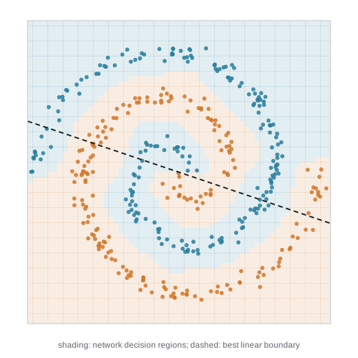
After 3,000 full-batch steps the network classifies the training spirals almost perfectly, while the best linear classifier manages only about 63 per cent, little better than always guessing one side of a line through the middle. The network has 1,185 parameters, enough to bend its decision boundary around both arms but not wildly more than the 400 training points, and it has found a smooth representation in which the spirals unwind. Whether it generalizes to new points from the same spirals is a separate question; on such a smooth problem it does, but lesson 5 is about why that is not guaranteed.

What the rest of the course covers

Lessons 2 to 5 cover the general machinery: computing gradients by automatic differentiation, optimizers, initialization, normalization and residual connections, and regularization and generalization. Lessons 6 to 8 cover architectures that encode assumptions about data: convolutions for grids such as images, recurrence for sequences, and attention, which underlies the transformer. Lesson 9 covers pretraining, transfer and scaling laws, lesson 10 generative models, lesson 11 the practice of training and the interpretability and robustness of trained networks, and lesson 12 the responsibilities that come with the technology, ending with an end-to-end project. Applied depth lives elsewhere: AI-340 for language, AI-350 for vision, AI-410 for large language models, AI-480 for hardware and distributed training. This course is the core they all build on.

The examples use NumPy only, on deliberately tiny problems, because the goal is to understand the mechanisms. Real projects use a framework such as PyTorch or JAX, which provide automatic differentiation, GPU execution and libraries of layers. Everything implemented here by hand corresponds to a line or two in those frameworks, and knowing what that line does is what lets you debug it when it fails.

Worked examples