Regularization and generalization in deep networks

A modern network often has far more parameters than training examples, and lesson 1 noted that networks can approximate almost any function. Classical learning theory, as developed in CMPUT-367, would predict severe overfitting. Yet deep networks trained on real data generalize well, and the largest models often generalize best. This lesson covers the regularization techniques used in practice (weight decay, dropout, data augmentation, early stopping and their relatives) and then the puzzling evidence about generalization in deep learning: networks that memorize random labels, double descent, and the implicit regularization of gradient descent. The aim is to know which tools to reach for and to understand why the classical picture needs revising without being discarded.

Overfitting in networks

The symptoms are the familiar ones from CMPUT-367. Training loss keeps falling while validation loss reaches a minimum and rises; the gap between training and validation accuracy grows. The diagnosis tools are the same too: learning curves, a held-out validation set, and comparison with a simple baseline. What differs is that the remedies act on a model too large to analyse directly, and several of them work as much by changing the optimization as by limiting capacity.

Weight decay and norm penalties

An L2 penalty \(\frac{\lambda}{2}\lVert\theta\rVert^2\) adds \(\lambda\theta\) to the gradient and pulls every weight toward zero, preferring functions that use many small weights over a few large ones. For SGD this is identical to weight decay; for adaptive optimizers, lesson 3 showed that decoupled weight decay (AdamW) is the right form. Typical values are \(10^{-4}\) to \(5 \times 10^{-4}\) for convolutional networks trained with SGD and 0.01 to 0.1 for transformers trained with AdamW. Biases and normalization scales are usually excluded, because shrinking them does not reduce complexity in any useful sense.

In networks with normalization layers, weight decay plays a second role. A weight matrix followed by batch or layer normalization can be scaled by any positive constant without changing the network's function, so its norm does not measure complexity. Shrinking it does, however, increase the effective learning rate, because the same update is a larger relative change to a smaller matrix (Twan van Laarhoven, 2017; Guodong Zhang and colleagues, 2019). Weight decay in such networks is therefore partly a learning rate schedule in disguise, one reason its best value interacts with the learning rate.

Dropout

Dropout (Geoffrey Hinton and colleagues, 2012; Nitish Srivastava and colleagues, 2014) sets each hidden unit to zero with probability p on every training step, independently for each example. The network cannot rely on any particular unit being present, so it is pushed toward redundant, distributed features rather than fragile co-adaptations in which units only work in specific combinations. A network with n droppable units implicitly trains an ensemble of up to \(2^n\) thinned sub-networks that share weights; at test time all units are kept, which approximates averaging the ensemble's predictions.

For the expected activation to be the same in training and testing, outputs must be rescaled. The usual implementation, inverted dropout, multiplies surviving units by \(1/(1 - p)\) during training and does nothing at test time, so inference code needs no change. Typical rates are 0.5 for large fully connected layers, 0.1 to 0.3 elsewhere, and 0.1 in many transformers. Dropout is used less in convolutional layers, where neighbouring activations are strongly correlated, and spatial variants that drop whole channels work better there. Very large language models trained for a single pass over enormous data sets often use no dropout at all, because with that much data overfitting is not the binding constraint.

# Inverted dropout: drop units with probability p during training and rescale the survivors by 1/(1 - p).
import numpy as np
rng = np.random.default_rng(466)
h = rng.uniform(0.5, 1.5, size=(1, 10))          # one example's hidden activations
p = 0.5
def dropout(h, train):
    if not train:
        return h                                  # inference: no dropping, no rescaling needed
    mask = (rng.uniform(size=h.shape) >= p) / (1 - p)
    return h * mask
print("activations:        ", np.round(h, 2))
print("one training pass:  ", np.round(dropout(h, True), 2))
avg = np.mean([dropout(h, True) for _ in range(20000)], axis=0)
print("mean of 20,000 passes:", np.round(avg, 2))
print("max |mean - activation|:", round(float(np.abs(avg - h).max()), 3))

activations:         [[0.68 0.81 1.08 1.31 0.79 0.99 0.94 0.53 0.64 1.5 ]]
one training pass:   [[1.36 1.62 0.   0.   0.   1.97 1.89 0.   1.29 0.  ]]
mean of 20,000 passes: [[0.68 0.81 1.08 1.32 0.79 0.99 0.93 0.53 0.64 1.51]]
max |mean - activation|: 0.012

Monte Carlo dropout (Yarin Gal and Zoubin Ghahramani, 2016) keeps dropout on at test time and averages several stochastic forward passes; the spread of the predictions gives a rough measure of the model's uncertainty. It is cheap and widely used, though its estimates are often poorly calibrated compared with deep ensembles, which train several networks from different initializations (Balaji Lakshminarayanan and colleagues, 2017).

Data augmentation

The most effective regularizer is more data, and data augmentation manufactures it by applying transformations that should not change the label. For images: random crops, horizontal flips, small rotations, colour jitter, and stronger policies such as RandAugment. Mixup (Hongyi Zhang and colleagues, 2018) trains on convex combinations of pairs of examples and their labels, and CutMix pastes a patch of one image into another with labels mixed in proportion to area. For audio: time shifts, speed changes, added noise and SpecAugment's masking of time and frequency bands. For text, augmentation is harder because small edits can change meaning; back-translation (translating to another language and back) and token masking are common. Augmentation encodes knowledge about invariances, and choosing transformations that do not respect the task (flipping digits, for example, turns some 6s into near-9s) teaches the model the wrong invariance.

Early stopping

Early stopping monitors validation loss during training and keeps the parameters from the epoch where it was lowest, stopping when it has not improved for a chosen number of evaluations (the patience). For a quadratic loss trained by gradient descent from zero, early stopping is approximately equivalent to L2 regularization, with the number of steps times the learning rate playing the role of \(1/\lambda\) (Christopher Bishop, 1995): parameters along low-curvature directions, which are learned last, are the ones left small. It costs nothing and is almost always used, either explicitly or through a training budget chosen on validation data.

# Overfitting a small dataset with an MLP, and three remedies: weight decay, dropout and early stopping.
import numpy as np
def make(seed, n):
    r = np.random.default_rng(seed)
    X = r.uniform(-1, 1, (n, 2))
    y = ((X[:, 0] ** 2 + X[:, 1] ** 2 < 0.5) ^ (r.uniform(size=n) < 0.15)).astype(float)   # 15% label noise
    return X, y.reshape(-1, 1)
Xtr, ytr = make(1, 100); Xva, yva = make(2, 2000)
def train(decay=0.0, drop=0.0, epochs=2000, seed=466, H=64):
    r = np.random.default_rng(seed)
    W1 = r.normal(0, np.sqrt(2 / 2), (2, H)); b1 = np.zeros(H)
    W2 = r.normal(0, np.sqrt(2 / H), (H, H)); b2 = np.zeros(H)
    W3 = r.normal(0, np.sqrt(1 / H), (H, 1)); b3 = np.zeros(1)
    best = (1.0, 0); hist = []
    for ep in range(1, epochs + 1):
        h1 = np.maximum(0, Xtr @ W1 + b1)
        m1 = (r.uniform(size=h1.shape) >= drop) / (1 - drop); h1d = h1 * m1
        h2 = np.maximum(0, h1d @ W2 + b2)
        m2 = (r.uniform(size=h2.shape) >= drop) / (1 - drop); h2d = h2 * m2
        p = 1 / (1 + np.exp(-(h2d @ W3 + b3)))
        g = (p - ytr) / len(Xtr)
        gW3 = h2d.T @ g; g2 = (g @ W3.T) * m2 * (h2 > 0)
        gW2 = h1d.T @ g2; g1 = (g2 @ W2.T) * m1 * (h1 > 0)
        gW1 = Xtr.T @ g1
        lr = 0.5
        W3 -= lr * (gW3 + decay * W3); b3 -= lr * g.sum(0)
        W2 -= lr * (gW2 + decay * W2); b2 -= lr * g2.sum(0)
        W1 -= lr * (gW1 + decay * W1); b1 -= lr * g1.sum(0)
        if ep % 100 == 0:
            def err(X, y):
                q = np.maximum(0, np.maximum(0, X @ W1 + b1) @ W2 + b2) @ W3 + b3
                return np.mean((q > 0) != (y > 0.5))
            tr, va = err(Xtr, ytr), err(Xva, yva); hist.append((ep, tr, va))
            if va < best[0]: best = (va, ep)
    return hist, best
for name, kw in [("no regularization", {}), ("weight decay 1e-2", {"decay": 1e-2}), ("dropout 0.2", {"drop": 0.2})]:
    hist, best = train(**kw)
    ep, tr, va = hist[-1]
    print(f"{name:18} final: train error {tr:.3f}, validation error {va:.3f}; best validation {best[0]:.3f} at epoch {best[1]}")
print("Bayes error from label noise alone is about 0.15")

no regularization  final: train error 0.090, validation error 0.319; best validation 0.234 at epoch 300
weight decay 1e-2  final: train error 0.280, validation error 0.218; best validation 0.215 at epoch 1800
dropout 0.2        final: train error 0.140, validation error 0.372; best validation 0.274 at epoch 100
Bayes error from label noise alone is about 0.15

The unregularized network drives its training error well below the 15 per cent label noise, which means it has memorized wrong labels, and its validation error climbs after its best epoch, early in training. Early stopping at that epoch would have kept a validation error about 8 points lower than the final one. Weight decay at this strength is heavy-handed: training error stays well above the noise level, a sign of some underfitting, yet it gives the lowest final validation error, with almost no gap between its best and final epochs, so it is far less sensitive to when training stops. Dropout, on the other hand, makes things worse here. With only two input features and 64 hidden units, randomly removing units mostly injects noise into a model that has little redundancy to exploit; dropout earns its keep in large networks with many correlated features, where co-adaptation is a real risk. The lesson is general: regularizers are not interchangeable, and each must be validated on the problem at hand.

Other regularizers

Several other techniques regularize in practice. Label smoothing (lesson 2) penalizes overconfident logits. Stochastic depth (Gao Huang and colleagues, 2016) randomly skips whole residual blocks during training, a block-level dropout that also shortens training time. Batch normalization adds noise through batch statistics. Smaller batches and larger learning rates add gradient noise that tends to find flatter minima. Ensembles of independently trained networks are the most reliable way to improve accuracy and calibration, at a cost proportional to their size; averaging weights along a training trajectory (stochastic weight averaging, Pavel Izmailov and colleagues, 2018) or keeping an exponential moving average of the weights gets some of the benefit at almost no cost, and the moving average is standard in diffusion model training.

Rethinking generalization

In 2017 Chiyuan Zhang, Samy Bengio, Moritz Hardt, Benjamin Recht and Oriol Vinyals reported a simple experiment with large consequences. Standard image classification networks trained on CIFAR-10 with the labels randomly shuffled still reached 100 per cent training accuracy, taking only a few times longer than on the true labels. With true labels the same networks generalized well; with random labels, of course, they were at chance on test data. Explicit regularizers changed this little. The conclusion was that the capacity of these networks, as measured by their ability to fit arbitrary labels, is large enough that classical capacity-based bounds such as VC dimension are vacuous for them, and that whatever makes them generalize must depend on the data and on the training algorithm, not just the model class.

# Memorization: the same network fits real labels and randomly shuffled labels on 200 points.
import numpy as np
rng = np.random.default_rng(466)
X = rng.normal(size=(200, 20)); w = rng.normal(size=20)
y_real = (X @ w > 0).astype(float).reshape(-1, 1)
y_rand = rng.permutation(y_real.ravel()).reshape(-1, 1)     # labels no longer related to X
Xte = rng.normal(size=(2000, 20)); yte = (Xte @ w > 0).astype(float).reshape(-1, 1)
def fit(y, steps=2000):
    r = np.random.default_rng(1)
    W1 = r.normal(0, np.sqrt(2 / 20), (20, 128)); W2 = r.normal(0, np.sqrt(1 / 128), (128, 1))
    for t in range(1, steps + 1):
        h = np.maximum(0, X @ W1); p = 1 / (1 + np.exp(-(h @ W2)))
        g = (p - y) / len(X)
        gW2 = h.T @ g; gW1 = X.T @ ((g @ W2.T) * (h > 0))
        W1 -= 0.5 * gW1; W2 -= 0.5 * gW2
        if t in (200, 2000):
            acc = np.mean((p > 0.5) == y)
            test = np.mean(((np.maximum(0, Xte @ W1) @ W2) > 0) == yte)
            print(f"  step {t:4}: training accuracy {acc:.3f}, accuracy on fresh real-labelled data {test:.3f}")
print("real labels:"); fit(y_real)
print("shuffled labels:"); fit(y_rand)

real labels:
  step  200: training accuracy 1.000, accuracy on fresh real-labelled data 0.927
  step 2000: training accuracy 1.000, accuracy on fresh real-labelled data 0.926
shuffled labels:
  step  200: training accuracy 1.000, accuracy on fresh real-labelled data 0.427
  step 2000: training accuracy 1.000, accuracy on fresh real-labelled data 0.427

Double descent

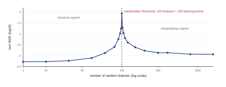
Classical theory pictures test error as a U-shaped function of model capacity: falling as bias drops, then rising as variance grows. Mikhail Belkin, Daniel Hsu, Siyuan Ma and Soumik Mandal (2019) showed that if capacity keeps increasing past the point where the model can exactly fit (interpolate) the training data, test error often peaks at that interpolation threshold and then falls again, sometimes below the classical minimum. Preetum Nakkiran and colleagues at OpenAI (2020) observed this double descent in convolutional networks and transformers as a function of width, of training time, and even of training set size.

The mechanism is clearest in linear regression on random features. Below the threshold, least squares has a unique solution. Exactly at the threshold, with as many features as data points, the system is just barely solvable, the solution must contort itself to hit every noisy target, and its norm, and with it the variance, blows up. Past the threshold, infinitely many solutions interpolate the data, and the minimum-norm one, which gradient descent from zero converges to, becomes smoother as more features are added, because the norm can be spread across more directions.

# Double descent with random ReLU features: test error of the minimum-norm least-squares fit
# as the number of features passes the number of training points (n = 100).
import numpy as np
rng = np.random.default_rng(466)
d, n, ntest = 10, 100, 2000
w_true = rng.normal(size=d) / np.sqrt(d)
def data(m):
    X = rng.normal(size=(m, d))
    return X, np.sin(2 * X @ w_true) + rng.normal(0, 0.2, m)
Xtr, ytr = data(n); Xte, yte = data(ntest)
for p in (10, 40, 80, 95, 100, 105, 120, 200, 400, 1600):
    errs = []
    for rep in range(10):                          # average over draws of the random features
        V = rng.normal(size=(d, p)) / np.sqrt(d)
        Ftr, Fte = np.maximum(0, Xtr @ V), np.maximum(0, Xte @ V)
        beta = np.linalg.pinv(Ftr) @ ytr           # minimum-norm solution once p >= n
        errs.append(np.mean((Fte @ beta - yte) ** 2))
    tag = "  <- interpolation threshold" if p == n else ""
    print(f"{p:5} features: median test MSE {np.median(errs):9.3f}{tag}")

   10 features: median test MSE     0.538
   40 features: median test MSE     0.861
   80 features: median test MSE     2.517
   95 features: median test MSE     7.256
  100 features: median test MSE    94.867  <- interpolation threshold
  105 features: median test MSE    11.905
  120 features: median test MSE     3.651
  200 features: median test MSE     1.689
  400 features: median test MSE     1.301
 1600 features: median test MSE     1.133

Implicit regularization and flat minima

If the model class can fit anything, the choice among the many interpolating solutions is made by the training procedure. This is implicit regularization. For linear models, gradient descent from zero converges to the minimum-norm interpolating solution, as in the double descent example; for logistic regression on separable data it converges in direction to the maximum-margin classifier (Daniel Soudry and colleagues, 2018). For deep networks the bias is harder to characterize, but evidence points to a preference for simple functions: networks learn low-frequency, smooth components of a target first (the spectral bias of Nasim Rahaman and colleagues, 2019), and SGD noise favours wide, flat minima, which several analyses connect to robustness and generalization, although sharpness depends on parameterization and is not by itself a reliable predictor.

Two other lines of theory give more meaningful bounds than VC dimension. PAC-Bayes bounds measure how much a network's weights can be perturbed without hurting its training loss, and Gintare Karolina Dziugaite and Daniel Roy (2017) obtained non-vacuous bounds for small image networks by optimizing them directly. The neural tangent kernel (Arthur Jacot, Franck Gabriel and Clément Hongler, 2018) shows that in the limit of infinite width, with a particular scaling, gradient descent on a network behaves like kernel regression with a fixed kernel; real networks of finite width learn features and depart from this regime, which is part of why they outperform kernels. No theory yet fully explains deep learning's generalization, and it remains one of the field's central open questions.

Practical guidance

In practice: start with a model large enough to overfit, then regularize. Use AdamW with moderate weight decay, data augmentation suited to the domain, early stopping on validation loss, and dropout or stochastic depth if overfitting persists. Keep an exponential moving average of the weights when training is noisy. Compare against a smaller model and a simple baseline, and remember that the strongest regularizer is more, cleaner data. The capacity arguments of CMPUT-367 still apply at the margin, but in deep learning the useful question is less how many parameters a model has than how the data, the architecture and the training procedure together select a solution.

Worked examples