CPU scheduling

At any moment a computer may have hundreds of threads that are ready to run and only a few cores to run them on. The scheduler is the part of the kernel that decides which ready thread runs next, on which core and for how long. Its decisions shape how a computer feels: whether the mouse pointer stays smooth while a compile runs in the background, whether a database meets its response-time targets, whether a car's brake controller always meets its deadlines. This lesson studies classic scheduling algorithms with simulations, then looks at what real kernels do, including Linux's fair schedulers and real-time scheduling.

Scheduling applies to threads, which Lesson 3 showed are the units the kernel actually runs; older texts say 'process scheduling' because early systems had one thread per process. We use 'job', 'task' and 'thread' loosely here to mean a schedulable unit.

CPU bursts and what we want to optimize

Programs alternate between CPU bursts, periods of computing, and input-and-output bursts, periods of waiting. Most bursts are short: an interactive program computes for a millisecond in response to a keystroke and then waits again. A few programs, such as video encoders and scientific simulations, have long CPU bursts. Good schedulers favour short bursts so that interactive programs respond quickly, while still giving long-running jobs their fair share.

Classic algorithms

First-come, first-served (FCFS) runs jobs in arrival order until each finishes. It is simple and fair in one sense, but short jobs stuck behind a long one wait a long time, the convoy effect. Shortest job first (SJF) always runs the job with the shortest next CPU burst, which provably minimizes average waiting time for a fixed set of jobs. Its preemptive version, shortest remaining time first (SRTF), switches to a newly arrived job if it is shorter than what remains of the current one. Both need to know burst lengths in advance; real schedulers can only estimate them, typically with an exponential average of past bursts, and long jobs can starve if short ones keep arriving.

Round robin (RR) gives each ready job a fixed time slice, the quantum, in turn. When the quantum expires the timer interrupt preempts the job and puts it at the back of the queue. Response time is good, because every job runs within a bounded time, but turnaround can be worse than SJF. The quantum matters: too long and RR becomes FCFS; too short and the processor spends much of its time on context switches. Quanta of 1 to 100 ms are typical, compared with context-switch costs of a few microseconds.

# Simulate FCFS, SJF (non-preemptive), SRTF (preemptive SJF) and Round Robin on one CPU
jobs = [("A", 0, 8), ("B", 1, 4), ("C", 2, 9), ("D", 3, 5)]   # (name, arrival, burst) in ms

def simulate(policy, q=4):
    t, done, gantt = 0, {}, []
    remaining = {n: b for n, a, b in jobs}
    first_run = {}
    ready = []
    queue = []                                   # used by round robin
    arrived = set()
    current = None
    while len(done) < len(jobs):
        for n, a, b in jobs:                     # admit arrivals
            if a <= t and n not in arrived:
                arrived.add(n); ready.append(n); queue.append(n)
        avail = [n for n in ready if n not in done]
        if not avail:
            t += 1; continue
        if policy == "FCFS":
            pick = min(avail, key=lambda n: dict((x[0], x[1]) for x in jobs)[n]); run = remaining[pick]
        elif policy == "SJF":
            pick = current if current in avail else min(avail, key=lambda n: (remaining[n], n)); run = remaining[pick]
        elif policy == "SRTF":
            pick = min(avail, key=lambda n: (remaining[n], n)); run = 1
        else:                                    # Round Robin with quantum q
            pick = queue.pop(0); run = min(q, remaining[pick])
        first_run.setdefault(pick, t)
        for _ in range(run):                     # run one ms at a time so arrivals join the queue in order
            if gantt and gantt[-1][0] == pick: gantt[-1][2] += 1
            else: gantt.append([pick, t, t + 1])
            gantt[-1][2] = t + 1
            t += 1; remaining[pick] -= 1
            for n, a, b in jobs:
                if a <= t and n not in arrived:
                    arrived.add(n); ready.append(n); queue.append(n)
        current = pick
        if remaining[pick] == 0:
            done[pick] = t
        elif policy == "RR":
            queue.append(pick)
    arr = {n: a for n, a, b in jobs}; burst = {n: b for n, a, b in jobs}
    tat = {n: done[n] - arr[n] for n in done}
    wait = {n: tat[n] - burst[n] for n in done}
    resp = {n: first_run[n] - arr[n] for n in done}
    chart = " ".join(f"{p}[{s}-{e}]" for p, s, e in gantt)
    avg = lambda d: sum(d.values()) / len(d)
    return chart, avg(wait), avg(tat), avg(resp)

for pol in ("FCFS", "SJF", "SRTF", "RR"):
    chart, w, ta, r = simulate(pol)
    print(f"{pol:<4} {chart}")
    print(f"     avg wait {w:5.2f}  avg turnaround {ta:5.2f}  avg response {r:5.2f}")

FCFS A[0-8] B[8-12] C[12-21] D[21-26]
     avg wait  8.75  avg turnaround 15.25  avg response  8.75
SJF  A[0-8] B[8-12] D[12-17] C[17-26]
     avg wait  7.75  avg turnaround 14.25  avg response  7.75
SRTF A[0-1] B[1-5] D[5-10] A[10-17] C[17-26]
     avg wait  6.50  avg turnaround 13.00  avg response  4.25
RR   A[0-4] B[4-8] C[8-12] D[12-16] A[16-20] C[20-24] D[24-25] C[25-26]
     avg wait 11.75  avg turnaround 18.25  avg response  4.50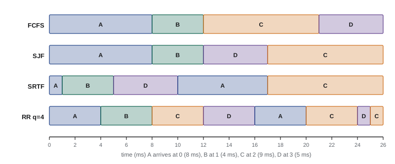

The simulation confirms the theory. SRTF has the lowest average waiting time (6.5 ms), SJF is next (7.75 ms) and FCFS is worse (8.75 ms) because B and D wait behind A and C. Round robin has the worst average waiting and turnaround times here, but its average response time (4.5 ms) is nearly as good as SRTF's (4.25 ms), and unlike SRTF it guarantees every job a turn within a bounded time whatever the burst lengths, without needing to know them. No single policy wins on every criterion, which is why real schedulers combine ideas.

Priorities, starvation and aging

Priority scheduling runs the highest-priority ready job. Priorities can reflect importance (a payment system above a report generator), user choice (the Unix nice value), or behaviour (interactive jobs above batch jobs). The danger is starvation: a low-priority job may never run if higher-priority work keeps arriving. Aging prevents this by gradually raising the priority of jobs that have waited a long time. A famous illustration: when MIT's IBM 7094 was shut down in 1973, administrators reportedly found a low-priority job submitted in 1967 that had never run.

Priority inversion is a subtler problem. A high-priority task waits for a lock held by a low-priority task, and a medium-priority task, which needs neither, preempts the low-priority task, so the high-priority task waits indefinitely. In 1997 this caused repeated resets on NASA's Mars Pathfinder lander until engineers enabled priority inheritance remotely: while a low-priority task holds a lock that a high-priority task needs, it temporarily inherits the higher priority. Lesson 5 returns to locks.

Multilevel feedback queues

A multilevel feedback queue (MLFQ) learns each job's behaviour instead of needing burst lengths in advance. It keeps several queues with different priorities and quanta. New jobs start in the top queue with a short quantum. A job that uses its whole quantum is probably processor-bound, so it moves down to a lower-priority queue with a longer quantum. A job that blocks for input before its quantum ends stays where it is. Interactive jobs therefore float near the top and respond quickly, while long jobs sink and run in large chunks when nothing else needs the processor. To prevent starvation, an MLFQ periodically boosts every job back to the top.

# A three-level multilevel feedback queue: new jobs start at the top; using a full quantum demotes them
from collections import deque
QUANTA = [2, 4, 8]                      # ms per level
jobs = {"editor": [1, 1, 1, 1, 1, 1],   # many short CPU bursts (interactive)
        "compile": [30]}                # one long CPU burst (batch)
level = {j: 0 for j in jobs}
queues = [deque(jobs), deque(), deque()]
t, log = 0, []
while any(queues):
    lv = next(i for i, q in enumerate(queues) if q)
    j = queues[lv].popleft()
    burst = jobs[j][0]
    run = min(burst, QUANTA[lv])
    log.append(f"t={t:>2} {j:<7} L{lv} ran {run}")
    t += run; jobs[j][0] -= run
    if jobs[j][0] == 0:
        jobs[j].pop(0)
        if jobs[j]: queues[lv].append(j)        # gave up the CPU early: stays at its level
    else:
        level[j] = min(lv + 1, 2)               # used its whole quantum: demoted
        queues[level[j]].append(j)
for line in log[:12]: print(line)
print("...")
print("final levels:", level)

t= 0 editor  L0 ran 1
t= 1 compile L0 ran 2
t= 3 editor  L0 ran 1
t= 4 editor  L0 ran 1
t= 5 editor  L0 ran 1
t= 6 editor  L0 ran 1
t= 7 editor  L0 ran 1
t= 8 compile L1 ran 4
t=12 compile L2 ran 8
t=20 compile L2 ran 8
t=28 compile L2 ran 8
...
final levels: {'editor': 0, 'compile': 2}

Variants of MLFQ scheduled Unix, early Windows NT and macOS for decades. The design has weaknesses: a clever program can stay at high priority by blocking just before its quantum expires, so practical versions account for total processor use at each level rather than resetting on every block.

Fair-share scheduling in Linux

From 2007 to 2023 Linux used the Completely Fair Scheduler (CFS). Rather than fixed time slices, CFS tracks each task's virtual runtime, the processor time it has received scaled by its weight, and always runs the task with the smallest virtual runtime, kept in a red-black tree ordered by that value. A task's weight comes from its nice value: each step of nice changes the share by about 10 per cent, from weight 88,761 at nice -20 to 15 at nice 19. Tasks that sleep a lot have low virtual runtime when they wake, so they run promptly, which gives interactive programs good response without explicit priority tricks.

# Linux CFS idea: run the task with the smallest virtual runtime; vruntime grows more slowly for heavier weights
import heapq
weights = {"nice -5 (video)": 3121, "nice 0 (browser)": 1024, "nice 10 (backup)": 110}  # from the kernel's table
vrt = {t: 0.0 for t in weights}
cpu = {t: 0 for t in weights}
heap = [(0.0, t) for t in weights]; heapq.heapify(heap)
SLICE = 1                                         # ms per decision in this toy model
for _ in range(1000):
    v, task = heapq.heappop(heap)
    cpu[task] += SLICE
    vrt[task] += SLICE * 1024 / weights[task]     # heavier weight -> vruntime advances more slowly
    heapq.heappush(heap, (vrt[task], task))
total = sum(cpu.values())
for task in weights:
    share = weights[task] / sum(weights.values())
    print(f"{task:<17} weight {weights[task]:>4}  CPU {cpu[task]:>4} ms  ({100*cpu[task]/total:5.1f}%, ideal {100*share:5.1f}%)")

nice -5 (video)   weight 3121  CPU  733 ms  ( 73.3%, ideal  73.3%)
nice 0 (browser)  weight 1024  CPU  241 ms  ( 24.1%, ideal  24.1%)
nice 10 (backup)  weight  110  CPU   26 ms  (  2.6%, ideal   2.6%)

Linux 6.6 (October 2023) replaced CFS with EEVDF, Earliest Eligible Virtual Deadline First. It keeps the idea of weighted fair shares but adds a virtual deadline to each task, which lets latency-sensitive tasks request shorter slices and get them sooner without taking more than their share overall. Linux also lets administrators group tasks with control groups (cgroups), so that, for example, each container or each user gets a fair share of the processor regardless of how many threads it runs. Lesson 12 uses cgroups again for containers.

Multiprocessor scheduling

With many cores, the scheduler must also decide where each task runs. Moving a task between cores loses the warm contents of its caches, so schedulers prefer processor affinity, keeping a task on the core where it last ran. Each core usually has its own run queue, which avoids a global lock, and a load balancer periodically moves tasks from busy cores to idle ones. On large servers with non-uniform memory access (NUMA), memory attached to one socket is faster for that socket's cores, so the scheduler also tries to keep tasks near their memory. Modern laptop and phone processors add heterogeneous cores, such as Arm's big.LITTLE designs and Intel's performance and efficiency cores, so the scheduler must also decide which tasks deserve the fast, power-hungry cores.

Real-time scheduling

In a real-time system, a correct result delivered late is a wrong result. Hard real-time tasks, such as airbag deployment or motor control, must never miss deadlines; soft real-time tasks, such as video playback, tolerate occasional misses. Two classic algorithms schedule periodic tasks, each with a computation time C and period T. Rate-monotonic (RM) scheduling gives fixed priorities, with shorter periods getting higher priority. Liu and Layland proved in 1973 that RM meets all deadlines if total utilization U, the sum of C/T, is at most n(2^(1/n) - 1), which falls towards about 69 per cent as the number of tasks grows. Earliest deadline first (EDF) uses dynamic priorities, always running the job whose deadline is soonest, and meets all deadlines whenever U is at most 1.

# Real-time schedulability: Liu and Layland bound for rate-monotonic, and EDF's utilization test
import math
tasks = [("brake sensor", 1, 5), ("motor control", 2, 10), ("telemetry", 4, 20)]   # (name, C, T) in ms
U = sum(c / t for _, c, t in tasks)
n = len(tasks)
bound = n * (2 ** (1 / n) - 1)
print(f"utilization U = {U:.3f}")
print(f"RM bound for n={n}: {bound:.3f} -> {'schedulable by the bound' if U <= bound else 'bound inconclusive'}")
print(f"EDF test U <= 1: {'schedulable' if U <= 1 else 'not schedulable'}")
# exact check by simulating EDF over the hyperperiod
H = math.lcm(*[t for _, _, t in tasks])
missed = 0; jobs = []
for t in range(H):
    for name, c, p in tasks:
        if t % p == 0: jobs.append([t + p, c, name])
    jobs = [j for j in jobs if j[1] > 0]
    if jobs:
        jobs.sort(); jobs[0][1] -= 1
    missed += sum(1 for j in jobs if j[0] <= t + 1 and j[1] > 0)
print(f"EDF simulation over hyperperiod {H} ms: {missed} deadline misses")

utilization U = 0.600
RM bound for n=3: 0.780 -> schedulable by the bound
EDF test U <= 1: schedulable
EDF simulation over hyperperiod 20 ms: 0 deadline misses

Linux supports real-time policies alongside its fair scheduler: SCHED_FIFO and SCHED_RR give fixed priorities that always beat normal tasks, and SCHED_DEADLINE implements EDF with admission control, refusing tasks that would make the system unschedulable. Since Linux 6.12 (2024), the PREEMPT_RT patches that make almost all kernel code preemptible are part of the mainline kernel, which narrowed the gap with dedicated real-time operating systems. Safety-critical systems still often use certified real-time kernels whose worst-case timing has been analysed.

Worked examples