
CMPUT-313 · Lesson 9 of 12 · 33 min
The network layer II: the control plane
Lesson 8 showed how a router forwards a packet once it has a forwarding table. This lesson asks where the tables come from. Routing algorithms compute good paths through a network of routers, and routing protocols carry the information those algorithms need. Inside a single network, routers use link-state protocols such as OSPF or distance-vector protocols, which look for least-cost paths. Between the networks that make up the internet, routers use BGP, which is driven less by cost than by business relationships and policy. We study both families, run the algorithms in code, see how routing can go wrong, and finish with software-defined networking, which moves the control plane into a logically centralized controller. CISSP-113 lesson 10 discusses BGP hijacking and other routing attacks; here we study how routing works.
The routing problem
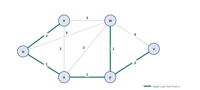
Routing algorithms model a network as a graph: routers are nodes, links are edges, and each link has a cost, which might reflect its length, its delay, its monetary cost or simply be inversely related to its capacity. The goal is to find a least-cost path from each source to each destination. Algorithms can be classified in several ways. A centralized, or global, algorithm computes paths with complete knowledge of the network's topology and link costs; link-state algorithms work this way. A decentralized algorithm computes paths iteratively, each router knowing only its neighbours and the information they send it; distance-vector algorithms work this way. Algorithms can also be static or dynamic, and load-sensitive or not; internet routing protocols are dynamic but deliberately not load-sensitive, because chasing congestion causes routes to oscillate.
Link-state routing and Dijkstra's algorithm
In link-state routing, every router learns the full topology. Each router floods a link-state advertisement describing its links and their costs to every other router, so that all routers build identical maps. Each then runs Dijkstra's algorithm, which CMPUT-204 lesson 9 analysed, to compute least-cost paths from itself to every destination, and installs the first hop of each path in its forwarding table. Dijkstra's algorithm grows a set of nodes whose least-cost paths are known, at each step adding the closest node not yet in the set and updating its neighbours' distances. With a heap it runs in \(O((E + N)\log N)\) time for \(N\) nodes and \(E\) links.
graph = {   # undirected link costs for the six-router example network
    "u": {"v": 2, "x": 1, "w": 5}, "v": {"u": 2, "x": 2, "w": 3}, "x": {"u": 1, "v": 2, "w": 3, "y": 1},
    "w": {"u": 5, "v": 3, "x": 3, "y": 1, "z": 5}, "y": {"x": 1, "w": 1, "z": 2}, "z": {"w": 5, "y": 2},
}
import heapq
def dijkstra(src):
    dist, prev, done = {src: 0}, {}, set()
    pq = [(0, src)]
    while pq:
        d, n = heapq.heappop(pq)
        if n in done:
            continue
        done.add(n)
        for m, c in graph[n].items():
            if d + c < dist.get(m, float("inf")):
                dist[m], prev[m] = d + c, n
                heapq.heappush(pq, (d + c, m))
    return dist, prev
dist, prev = dijkstra("u")
print("dest  cost  path            first hop")
for dest in sorted(dist):
    if dest == "u":
        continue
    path, n = [dest], dest
    while n != "u":
        n = prev[n]; path.append(n)
    path.reverse()
print(f" {dest} {dist[dest]} {'-'.join(path):14s} {path[1]}")dest cost path first hop v 2 u-v v w 3 u-x-y-w x x 1 u-x x y 2 u-x-y x z 4 u-x-y-z x
The first-hop column is exactly what router u puts in its forwarding table: packets to y, w or z leave on the link to x. One hazard of link-state routing with load-sensitive costs is oscillation: if link costs reflect current traffic, all routers move their traffic to the least-loaded path at once, making it the most loaded, and the routes flap back and forth. Real link-state protocols avoid this by using costs that do not depend on load, and by having routers run their computations at different moments.
Distance-vector routing and Bellman–Ford
In distance-vector routing, no router knows the whole topology. Each router keeps a vector of its estimated least costs to every destination and sends it to its neighbours from time to time and whenever it changes. When router \(x\) receives its neighbours' vectors, it updates its own estimates with the Bellman–Ford equation: the least cost from \(x\) to \(y\) is the minimum, over all neighbours \(v\), of the cost of the link to \(v\) plus \(v\)'s estimated cost to \(y\).
The algorithm is iterative, asynchronous and distributed, and it converges to the correct least costs as long as link costs stay fixed. The simulation below runs it synchronously on the same example network: in each round every router recomputes its vector from its neighbours' previous vectors. After a few rounds, u's vector matches the costs Dijkstra found.
graph = {   # undirected link costs for the six-router example network
    "u": {"v": 2, "x": 1, "w": 5}, "v": {"u": 2, "x": 2, "w": 3}, "x": {"u": 1, "v": 2, "w": 3, "y": 1},
    "w": {"u": 5, "v": 3, "x": 3, "y": 1, "z": 5}, "y": {"x": 1, "w": 1, "z": 2}, "z": {"w": 5, "y": 2},
}
# Distance-vector routing: every node repeatedly applies the Bellman-Ford equation
nodes = sorted(graph)
INF = float("inf")
D = {n: {m: (0 if m == n else graph[n].get(m, INF)) for m in nodes} for n in nodes}
for rnd in range(1, 10):
    new = {n: {m: 0 if m == n else min(graph[n][v] + D[v][m] for v in graph[n]) for m in nodes} for n in nodes}
    changed = sum(new[n][m] != D[n][m] for n in nodes for m in nodes)
    D = new
    print(f"round {rnd}: {changed:2d} entries changed;  u's vector:", {m: D['u'][m] for m in nodes})
    if not changed:
breakround 1: 16 entries changed; u's vector: {'u': 0, 'v': 2, 'w': 4, 'x': 1, 'y': 2, 'z': 10}
round 2: 6 entries changed; u's vector: {'u': 0, 'v': 2, 'w': 3, 'x': 1, 'y': 2, 'z': 4}
round 3: 0 entries changed; u's vector: {'u': 0, 'v': 2, 'w': 3, 'x': 1, 'y': 2, 'z': 4}When distance vector goes wrong: counting to infinity
Good news travels fast in distance-vector routing: when a link cost falls, the improvement spreads in a few rounds. Bad news travels slowly. Suppose routers x, y and z form a line, with link costs x–y of 4 and y–z of 1, so z reaches x through y at cost 5. If the x–y link cost rises to 60, y looks for a better route and sees that z advertises cost 5 to x, not realizing that z's route goes through y itself. So y switches to the route via z at cost 6 and tells z, which updates its cost to 7 and tells y, and the two routers ping-pong their costs upward one step at a time until y's route via z finally exceeds the direct cost of 60. If the link fails entirely, they count all the way up to the value that represents infinity. Meanwhile, packets for x loop between y and z.
# Count to infinity: routers x - y - z in a line; link x-y has cost 4, link y-z cost 1.
# Distances to x: y = 4 (direct), z = 5 (via y). Then the x-y link cost rises to 60.
def converge(poisoned_reverse):
    c_yx, c_yz = 60, 1
    Dy, Dz = 4, 5
    exchanges = 0
    while True:
        # z's route to x goes through y, so with poisoned reverse z tells y "infinity"
        z_says = float("inf") if poisoned_reverse else Dz
        new_Dy = min(c_yx, c_yz + z_says)
        new_Dz = c_yz + new_Dy            # z's only route to x is through y
        if (new_Dy, new_Dz) == (Dy, Dz):
            return exchanges, Dy
        Dy, Dz = new_Dy, new_Dz
        exchanges += 1
        if exchanges <= 3 or not poisoned_reverse and exchanges % 10 == 0:
            print(f"  exchange {exchanges:2d}: y's cost to x = {Dy}, z's cost to x = {Dz}")
print("without poisoned reverse:")
n, final = converge(False)
print(f"  {n} exchanges before y settles on cost {final}")
print("with poisoned reverse:")
n, final = converge(True)
print(f" {n} exchange before y settles on cost {final}")without poisoned reverse: exchange 1: y's cost to x = 6, z's cost to x = 7 exchange 2: y's cost to x = 8, z's cost to x = 9 exchange 3: y's cost to x = 10, z's cost to x = 11 exchange 10: y's cost to x = 24, z's cost to x = 25 exchange 20: y's cost to x = 44, z's cost to x = 45 28 exchanges before y settles on cost 60 with poisoned reverse: exchange 1: y's cost to x = 60, z's cost to x = 61 1 exchange before y settles on cost 60
A partial fix is poisoned reverse: if z routes to x through y, z tells y that its distance to x is infinite, so y will never route back through z. This solves loops between two neighbours but not loops involving three or more routers. The Routing Information Protocol (RIP), an early distance-vector protocol, limits infinity to 16 hops for this reason, which restricts it to small networks. Modern distance-vector protocols such as Babel and Cisco's EIGRP use additional mechanisms to guarantee loop freedom.
| Property | Link state (OSPF, IS-IS) | Distance vector (RIP, Babel) |
|---|---|---|
| What a router knows | The full topology | Only its neighbours' distance vectors |
| Messages | Link-state advertisements flooded to all routers | Distance vectors sent to neighbours |
| Computation | Dijkstra on the whole graph | Bellman–Ford updates |
| Convergence | Fast once advertisements are flooded | Can be slow; may count to infinity |
| Robustness to a faulty router | A bad advertisement affects only that router's links | A bad vector can spread through the network |
Routing inside an autonomous system: OSPF
The internet is not one flat network that could run a single routing algorithm: there are too many routers, and each organization wants to control its own network. Instead, routers are grouped into autonomous systems (ASes), each a network under one administration with a globally unique AS number. Within an AS, routers run an intra-AS routing protocol, also called an interior gateway protocol. The most common are OSPF (Open Shortest Path First, RFC 2328 for IPv4) and IS-IS, both link-state protocols. OSPF floods link-state advertisements whenever a link changes and refreshes them periodically, authenticates messages so that intruders cannot inject false routes, can use several equal-cost paths at once, and supports a hierarchy of areas connected by a backbone area, so that each router needs detailed topology only for its own area. Network operators choose link weights to steer traffic, a task called traffic engineering.
Worked problem
Setting OSPF weights to steer traffic
In the example network, operators want traffic from u to z to avoid the x–y link, which is reserved for a backup data feed. Which single link weight change achieves this, and what is the new path?
Show solution
- Currently u to z goes u-x-y-z at cost 4.
- Raise the x–y weight from 1 to 10. Now the candidates are u-x-w-y-z (1 + 3 + 1 + 2 = 7), u-v-w-y-z (2 + 3 + 1 + 2 = 8), u-w-y-z (5 + 1 + 2 = 8) and u-x-y-z (1 + 10 + 2 = 13).
- The new least-cost path is u-x-w-y-z at cost 7, which avoids x–y.
- Weight changes affect all traffic that used the link, so operators simulate the whole traffic matrix before changing them.
Answer: Raise the x–y weight (for example to 10); u to z then follows u-x-w-y-z at cost 7.
Routing between autonomous systems: BGP
The Border Gateway Protocol, version 4 (BGP, RFC 4271), is the glue that holds the internet together. About 75,000 autonomous systems were active in 2025, and every one uses BGP to tell its neighbours which address prefixes it can reach. BGP is a path-vector protocol: each advertisement for a prefix carries the AS-PATH attribute, the list of ASes the advertisement has passed through, and the NEXT-HOP attribute, the address of the router to send packets to. AS-PATH lets a router detect and reject loops: it ignores any advertisement whose path already contains its own AS number. BGP sessions run over TCP port 179. External BGP (eBGP) sessions connect routers in different ASes; internal BGP (iBGP) sessions spread the learned routes to all routers inside an AS, which combine them with their intra-AS routes to reach the exit points.
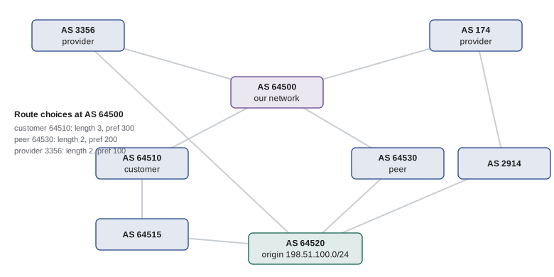
When a router learns several routes to the same prefix, it chooses one by applying rules in order: highest local preference, a value set by the AS's own policy; then shortest AS-PATH; then the closest NEXT-HOP router according to intra-AS routing, called hot-potato routing because it hands the packet to another AS as soon as possible; then further tie-breakers. Policy dominates. An AS sets local preference to favour routes through customers, who pay it, over routes through peers, which cost nothing, over routes through providers, which it pays. Export policy follows the same economics, an arrangement analysed by Gao and Rexford: an AS advertises routes learned from customers to everyone, but routes learned from peers or providers only to its customers, so it never carries traffic between two networks that do not pay it.
# Simplified BGP route selection at AS 64500 for prefix 198.51.100.0/24
routes = [  # (learned from, relationship, AS path, MED)
    ("AS 64510", "customer", [64510, 64515, 64520], 0),
    ("AS 3356", "provider", [3356, 64520], 0),
    ("AS 64530", "peer", [64530, 64520], 0),
    ("AS 174", "provider", [174, 2914, 64520], 0),
]
local_pref = {"customer": 300, "peer": 200, "provider": 100}   # prefer routes that earn money
def key(r):
    return (-local_pref[r[1]], len(r[2]), r[3])                 # higher pref, shorter path, lower MED
for r in sorted(routes, key=key):
    print(f"{r[0]:9s} {r[1]:9s} pref {local_pref[r[1]]}  AS path {' '.join(map(str, r[2])):17s} length {len(r[2])}")
best = min(routes, key=key)
print("selected:", best[0], "- the customer route wins on local preference even though its path is longer")
# Export policy (Gao-Rexford): routes from peers or providers are told only to customers
for r in routes:
    tell = "customers, peers and providers" if r[1] == "customer" else "customers only"
print(f"a route learned from a {r[1]:8s} is exported to {tell}")AS 64510 customer pref 300 AS path 64510 64515 64520 length 3 AS 64530 peer pref 200 AS path 64530 64520 length 2 AS 3356 provider pref 100 AS path 3356 64520 length 2 AS 174 provider pref 100 AS path 174 2914 64520 length 3 selected: AS 64510 - the customer route wins on local preference even though its path is longer a route learned from a customer is exported to customers, peers and providers a route learned from a provider is exported to customers only a route learned from a peer is exported to customers only a route learned from a provider is exported to customers only
BGP has known weaknesses. Any AS can announce any prefix, so a misconfiguration or an attack can hijack traffic: in 2008 Pakistan Telecom accidentally redirected YouTube worldwide for about two hours, and route leaks still cause outages every year. The Resource Public Key Infrastructure (RPKI) lets address holders sign route origin authorizations, so that routers can reject announcements from the wrong origin AS; by 2025 roughly half of IPv4 routes were covered by such authorizations. BGPsec, which would sign entire paths, has seen little deployment. BGP also converges slowly after failures, sometimes taking minutes, and one router's change can ripple across the internet. CISSP-113 lesson 10 treats BGP security in more depth.
Worked problem
Why did the traffic go the long way?
A Canadian university AS has two providers: a national research network, set with local preference 200, and a commercial transit provider, set with local preference 100. A popular video service is reachable through the research network with AS path length 4 and through the commercial provider with length 2. Which route does the university choose, and why might students see higher delay?
Show solution
- BGP compares local preference first: 200 beats 100, so the research network route wins even though its AS path is longer.
- AS path length counts ASes, not kilometres or milliseconds; the longer path might also be geographically longer, or it might be faster.
- If the research network reaches the video service through a distant exchange, students may see higher delay than the commercial route would give.
- Operators can fix this by adjusting local preference for that prefix, or the video service can place a CDN cache inside the research network.
Answer: The research network route, because local preference outranks AS-path length; policy, not delay, decides BGP paths.
Software-defined networking
Traditionally, every router runs its own routing processes, and the control plane is distributed across the network. Software-defined networking (SDN) separates the control plane from the data plane: a logically centralized controller, which may itself run on a cluster of servers for reliability, computes forwarding rules and installs them in simple switches using a protocol such as OpenFlow, introduced in lesson 8. Network applications run on top of the controller: routing, load balancing, access control, traffic engineering. Because the controller sees the whole network, it can implement policies that are awkward with distributed protocols, such as routing different classes of traffic over different paths or reacting to failures with precomputed backup paths.
SDN is most successful where one organization controls the whole network. Google's B4 network, connecting its data centres, used SDN to run its wide-area links at close to full utilization by centrally allocating bandwidth among applications. Data centre networks and cloud providers' virtual networks, which CISSP-113 lesson 9 discusses, are built on SDN principles, and many enterprises now use SD-WAN products that apply them to their branch-office links. Across the public internet, between independent ASes, BGP remains the only way to route.
Common mistakes
MistakeThinking BGP chooses the shortest or fastest path.
InsteadBGP applies policy first, through local preference, and counts AS hops rather than delay.
MistakeAssuming distance-vector routers know the whole topology.
InsteadThey know only their neighbours' vectors; link-state routers know the whole topology.
MistakeUsing load-sensitive link costs naively.
InsteadCosts that follow traffic make routes oscillate; production protocols use stable weights.
MistakeBelieving poisoned reverse eliminates all routing loops.
InsteadIt stops two-node loops but not loops among three or more routers.
MistakeTreating an autonomous system as a single router.
InsteadAn AS is a whole network of routers under one administration, running intra-AS and inter-AS routing.
MistakeAssuming SDN replaces BGP on the internet.
InsteadSDN works within a network one organization controls; BGP still routes between autonomous systems.
Summary and key terms
- Routing computes paths in a graph whose links have costs; forwarding tables store each destination's first hop.
- Link-state routing floods topology to all routers, which run Dijkstra's algorithm.
- Distance-vector routing exchanges cost vectors with neighbours using the Bellman–Ford equation.
- Distance vector converges quickly on good news but can count to infinity on bad news; poisoned reverse helps only for two-node loops.
- Within an autonomous system, OSPF and IS-IS provide link-state routing with areas and traffic engineering.
- Between ASes, BGP advertises prefixes with AS paths, chooses routes by policy then path length, and exports routes according to business relationships.
- SDN centralizes control and installs match–action rules in switches, mainly within single organizations.
- Link-state routing
- Routing in which every router learns the full topology and computes paths itself.
- Dijkstra's algorithm
- A greedy algorithm that computes least-cost paths from one node to all others.
- Distance-vector routing
- Routing in which routers exchange estimated costs with neighbours and apply Bellman–Ford.
- Count to infinity
- Slow convergence of distance-vector routing after a cost increase, with temporary loops.
- Poisoned reverse
- Advertising an infinite cost to the neighbour through which a route passes.
- Autonomous system (AS)
- A network under a single administration, identified by an AS number.
- OSPF
- Open Shortest Path First, a link-state intra-AS routing protocol.
- BGP
- The Border Gateway Protocol, the path-vector protocol used between autonomous systems.
- AS-PATH
- The BGP attribute listing the ASes a route advertisement has traversed.
- Hot-potato routing
- Choosing the exit from your AS that is closest according to intra-AS routing.
Practice problems
Work each problem on paper first, then reveal the answer to check.
In the example network, what is the least cost from u to w and the path?
Show answer
Cost 3, via u-x-y-w.
State the Bellman–Ford equation.
Show answer
D_x(y) = min over neighbours v of c(x, v) + D_v(y).
Why does RIP set infinity to 16?
Show answer
To bound counting to infinity, which limits RIP to small networks.
What does a router do with a BGP advertisement whose AS path contains its own AS number?
Show answer
It rejects it to prevent a loop.
Which BGP attribute is compared first in route selection?
Show answer
Local preference.
Why would an AS not export a route learned from one provider to another provider?
Show answer
It would carry traffic between two networks it pays, earning nothing.
What is hot-potato routing?
Show answer
Sending traffic to the nearest exit from your own AS.
Give one advantage of link-state over distance-vector routing.
Show answer
Faster convergence, and a bad advertisement affects only one router's links.
What does RPKI protect against?
Show answer
Announcements of a prefix from an AS that is not authorized to originate it.
Where has SDN been most successful?
Show answer
In networks one organization controls, such as data centres and private wide-area networks.
Lesson quiz · 5 questions
Score 60% or more to complete this lesson.
Create a free account to save your progress, take quizzes and earn a certificate.