
CMPUT-313 · Lesson 1 of 12 · 40 min
The internet: structure, delay, loss and throughput
Almost every program you will write after this course talks to another program over a network. A phone app fetches data from a server, a game synchronizes players across a continent, a sensor on a robot streams readings to a control station, and the course page you are reading travelled to you as a few hundred packets. Computer networks are the systems that make this possible, and the internet is the largest and most important of them: a network of networks that connects billions of devices run by tens of thousands of independent organizations. This course looks at the internet from the computer scientist's point of view. We ask how its protocols work, why they were designed the way they were, and how well they perform. We will write programs that use sockets, build and parse real packet formats, and simulate the algorithms that decide how fast data may flow and which way it should go.
This first lesson builds the vocabulary and the quantitative tools the rest of the course depends on. We look at how the internet is put together, from the edge where hosts live to the core where routers forward packets, and we compare packet switching with circuit switching. Then we measure performance: the four components of delay, how queueing creates loss, what throughput means for a whole path, and how the bandwidth–delay product describes how much data is in flight. CISSP-113 covers the same structure from a security point of view, and DCE-210 looks at networking inside data centres; here the emphasis is on how and why the protocols behave as they do.
A network of networks
At the edge of the internet are the end systems, also called hosts: laptops, phones, servers, smart thermostats, cars and industrial controllers. Hosts run applications. They are connected to the network by access networks: home connections over cable, fibre or DSL, cellular networks, Wi-Fi in a campus or café, and Ethernet in an office or data centre. Inside the network are packet switches, chiefly routers (which forward packets based on network-layer addresses) and link-layer switches (which forward frames within a local network). Links connect everything: copper twisted pair, coaxial cable, optical fibre and radio.
No single company owns the internet. Hosts connect to an internet service provider (ISP), which may be a local or regional provider. Regional ISPs buy transit from larger ISPs, which in turn connect to a small number of global tier-1 networks that reach every part of the internet without paying anyone for transit. ISPs also connect directly to each other at internet exchange points (IXPs), where many networks meet in one building to exchange traffic, often without payment, an arrangement called peering. Large content providers such as video platforms and cloud companies run their own global networks and connect to ISPs at hundreds of IXPs, so that much of today's traffic never touches a tier-1 network at all. Canada has several IXPs, including TorIX in Toronto and YYCIX in Calgary, and the United States has dozens; the largest exchanges in the world move many terabits per second.
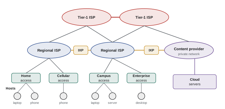
Two ideas hold this federation together. The first is a set of shared protocols. A protocol defines the format and order of messages exchanged between two or more communicating entities, and the actions taken when a message is sent or received or some other event occurs. The internet's protocols are specified in documents called Requests for Comments (RFCs), published by the Internet Engineering Task Force (IETF), an open standards body where anyone can participate. The second idea is the service model: the internet offers applications a simple, best-effort service for moving packets between hosts and leaves almost everything else, from reliability to security to congestion control, to the end systems. This end-to-end principle, argued by Saltzer, Reed and Clark in 1984, is one reason the internet could grow so quickly: new applications need only new software at the edges, not changes inside the network.
Packet switching and circuit switching
There are two basic ways to move data through a network of links and switches. In circuit switching, used by the traditional telephone network, resources along the path are reserved for the duration of a call. A circuit might be a time slot in each link's frame (time-division multiplexing) or a frequency band (frequency-division multiplexing). Once the circuit is set up, the sender gets a guaranteed constant rate and delay. The cost is that reserved capacity sits idle whenever the sender is silent.
In packet switching, used by the internet, a message is broken into packets, and each packet travels through the network independently, using the full rate of each link while it is being transmitted. Nothing is reserved. Most routers use store-and-forward transmission: a router must receive an entire packet before it begins to transmit it on the outgoing link. If packets arrive faster than an outgoing link can send them, they wait in an output queue, called a buffer. If the buffer is full, arriving packets are dropped. Packet switching therefore offers no guarantees, but it uses capacity far more efficiently for bursty traffic, which is what most computer traffic is.
The classic illustration compares the two for many users sharing a link. Suppose a 1 Gbit/s link is shared by users who each need 100 Mbit/s when active but are active only 10% of the time. Circuit switching can support exactly 10 users, because each must reserve 100 Mbit/s. With packet switching, 35 users can share the link and the chance that more than 10 are active at the same moment is tiny, so they almost always get their full rate. The worked example below computes this probability with the binomial distribution.
Worked problem
How many users can packet switching support?
A 1 Gbit/s link is shared by users who each transmit at 100 Mbit/s when active and are active independently 10% of the time. With circuit switching, how many users can be supported? With packet switching and 35 users, what is the probability that more than 10 are active at once?
Show solution
- Circuit switching reserves 100 Mbit/s per user, so the link supports \(1000/100 = 10\) users regardless of how often they are active.
- With packet switching, the number of active users among 35 follows a binomial distribution with \(n = 35\) and \(p = 0.1\). We need \(P(X > 10) = 1 - \sum_{k=0}^{10} \binom{35}{k} 0.1^k 0.9^{35-k}\).
from math import comb n, p = 35, 0.1 prob = 1 - sum(comb(n, k) * p**k * (1 - p)**(n - k) for k in range(11)) print(f'P(more than 10 of {n} active) = {prob:.6f}') for users in (35, 50, 60): q = 1 - sum(comb(users, k) * p**k * (1 - p)**(users - k) for k in range(11)) print(users, 'users:', f'{q:.4%}')- The probability is about 0.0004. Even with 50 users the link is overloaded less than 1% of the time; with 60 users overload becomes noticeably more common, and queues would build up.
Answer: Circuit switching supports 10 users. With packet switching, 35 users exceed the link capacity only about 0.04% of the time, so packet switching serves more than three times as many users with almost no loss of service.
The comparison is not entirely one-sided. Applications that need a steady rate with tight delay limits, such as a voice call over a congested link, would prefer reservations. The internet answers this mostly by overprovisioning links and by giving priority to some traffic in places where operators control both ends, rather than by reserving circuits end to end.
The four components of delay
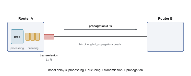
As a packet travels from one router to the next, it experiences four kinds of delay at each hop. Their sum is the nodal delay, and adding nodal delays along the path gives the end-to-end delay.
| Delay | Cause | Typical size | Depends on |
|---|---|---|---|
| Processing | Examining the header, checking for bit errors, looking up the outgoing link | Microseconds or less | Router hardware |
| Queueing | Waiting behind other packets in the output buffer | Zero to many milliseconds | Traffic intensity and burstiness |
| Transmission | Pushing all of the packet's bits onto the link | L/R: 1,500 bytes at 1 Gbit/s is 12 microseconds | Packet length L and link rate R |
| Propagation | A bit travelling along the medium from one end of the link to the other | d/s: about 5 microseconds per kilometre of fibre | Distance d and propagation speed s |
Students often confuse transmission delay with propagation delay. Transmission delay is the time to push the packet out of the router: it depends on the packet's length \(L\) and the link's rate \(R\), and has nothing to do with distance. Propagation delay is the time for one bit to travel the length of the link: it depends on the distance \(d\) and the propagation speed \(s\), which is about two thirds of the speed of light in fibre and copper, and has nothing to do with the packet's size. A useful analogy is a caravan of cars passing through a toll booth: the time for the booth to serve the whole caravan is like transmission delay, and the time for one car to drive to the next booth is like propagation delay.
The program below computes transmission and propagation delays for a packet crossing three very different links. Look at which delay dominates on each one: on the slow, short home link transmission dominates, while on the fast, long-haul fibre link propagation dominates by a factor of hundreds.
# Delay of one 1,500-byte packet over a path of three links
L = 1500 * 8                     # packet length in bits
links = [  # (name, rate in bit/s, length in m, propagation speed in m/s)
    ("home Wi-Fi to router", 100e6, 10, 3e8),
    ("access link to ISP", 50e6, 4_000, 2e8),
    ("long-haul optical link", 10e9, 1_200_000, 2e8),
]
total = 0.0
for name, R, d, s in links:
    d_trans = L / R
    d_prop = d / s
    total += d_trans + d_prop
    print(f"{name:22s} transmission {d_trans*1e3:8.4f} ms  propagation {d_prop*1e3:8.4f} ms")
print(f"end-to-end (no queueing, ignoring processing): {total*1e3:.3f} ms")home Wi-Fi to router transmission 0.1200 ms propagation 0.0000 ms access link to ISP transmission 0.2400 ms propagation 0.0200 ms long-haul optical link transmission 0.0012 ms propagation 6.0000 ms end-to-end (no queueing, ignoring processing): 6.381 ms
Queueing delay and packet loss
Queueing delay is the most interesting and least predictable component, because it depends on what other traffic is doing. Let \(a\) be the average rate at which packets arrive at an output queue, in packets per second, and suppose all packets are \(L\) bits long. The ratio \(La/R\) is the traffic intensity. If it is greater than 1, bits arrive faster than they can leave and the queue grows without limit, or rather until the buffer fills and packets are dropped. Even when the intensity is below 1, queueing delay depends on how bursty the arrivals are. If packets arrive perfectly evenly spaced, there is no queueing at all; if they arrive in bursts, the later packets in each burst must wait.
Queueing theory gives a simple model when arrivals are random (a Poisson process) and transmission times are exponentially distributed: the M/M/1 queue. Its mean waiting time is \(\rho/(1-\rho)\) service times, where \(\rho\) is the traffic intensity. BUS-230 used the same model for checkout lines and call centres. The striking feature is how sharply delay rises as intensity approaches 1: at 50% load a packet waits on average one packet time, at 90% nine, and at 99% ninety-nine.
# Average queueing delay grows sharply as traffic intensity approaches 1 (M/M/1 model)
R = 100e6          # link rate, bit/s
L = 1500 * 8       # average packet size, bits
service = L / R    # seconds to transmit one packet
for rho in (0.1, 0.5, 0.7, 0.8, 0.9, 0.95, 0.99):
    wait = rho / (1 - rho) * service          # mean time waiting in the queue
    print(f"intensity {rho:4.2f}: mean queueing delay {wait*1e6:9.1f} microseconds "
f"({rho/(1-rho):6.1f} packet times)")intensity 0.10: mean queueing delay 13.3 microseconds ( 0.1 packet times) intensity 0.50: mean queueing delay 120.0 microseconds ( 1.0 packet times) intensity 0.70: mean queueing delay 280.0 microseconds ( 2.3 packet times) intensity 0.80: mean queueing delay 480.0 microseconds ( 4.0 packet times) intensity 0.90: mean queueing delay 1080.0 microseconds ( 9.0 packet times) intensity 0.95: mean queueing delay 2280.0 microseconds ( 19.0 packet times) intensity 0.99: mean queueing delay 11880.0 microseconds ( 99.0 packet times)
Real routers have finite buffers. When a packet arrives to a full buffer it is dropped, and that packet is lost unless a higher layer, usually TCP, notices and retransmits it. The simulation below sends random traffic into a queue with room for 20 packets. At 60% load, loss is essentially zero. At 90% load, delay grows and some packets are lost. At 110% load, the queue stays nearly full: delay approaches the buffer size multiplied by the packet time, and roughly the excess traffic is dropped.
# Simulate a router queue with random arrivals and a finite buffer
import random
random.seed(313)
R, L = 10e6, 1500 * 8            # 10 Mbit/s link, 1,500-byte packets
service = L / R                  # 1.2 ms per packet
for rho, buffer in ((0.6, 20), (0.9, 20), (1.1, 20)):
    lam = rho / service           # arrival rate, packets per second
    t, free_at, queue, sent, dropped, delays = 0.0, 0.0, [], 0, 0, []
    for _ in range(200_000):
        t += random.expovariate(lam)
        queue = [d for d in queue if d > t]      # departure times still in the system
        if len(queue) >= buffer:
            dropped += 1
            continue
        start = max(t, free_at)
        free_at = start + service
        queue.append(free_at)
        delays.append(free_at - t)
        sent += 1
    loss = dropped / (sent + dropped)
print(f"intensity {rho:.1f}: loss {loss:6.2%}, mean delay {sum(delays)/len(delays)*1e3:6.2f} ms")intensity 0.6: loss 0.00%, mean delay 2.10 ms intensity 0.9: loss 0.18%, mean delay 6.04 ms intensity 1.1: loss 9.31%, mean delay 18.25 ms
How big should router buffers be? A long-standing rule of thumb set the buffer to the bandwidth–delay product of the link, so that a single TCP flow could keep the link busy. Research by Appenzeller, Keslassy and McKeown in 2004 showed that links carrying many flows need much less, roughly the bandwidth–delay product divided by the square root of the number of flows. Oversized buffers cause a problem called bufferbloat, where queues fill up and add hundreds of milliseconds of delay without improving throughput, which is painful for video calls and games. Modern active queue management algorithms such as CoDel and FQ-CoDel drop or mark packets early to keep queueing delay small; lesson 7 shows how TCP reacts to these signals.
Measuring delay in practice
The traceroute program, written by Van Jacobson in 1987, measures delay hop by hop. It sends packets with increasing values of the time-to-live (TTL) field in the IP header. Each router decrements the TTL and, when it reaches zero, discards the packet and returns an ICMP time-exceeded message to the sender. By sending three probes with TTL 1, three with TTL 2 and so on, traceroute learns the address of each router on the path and the round-trip time to it. Round-trip times do not always increase smoothly along the path: a router may be slow to generate ICMP replies, return traffic may follow a different path, and a long undersea or transcontinental link shows up as a sudden jump of tens of milliseconds. Lesson 8 returns to TTL and ICMP. The ping program is simpler: it sends ICMP echo requests and reports round-trip times and loss.
The round-trip time (RTT) between two hosts is one of the most important numbers in networking. Light in fibre covers about 200 kilometres per millisecond, so the propagation delay alone puts a floor under every RTT: roughly 34 ms for a round trip between Toronto and Vancouver along a 3,400 km fibre route, and more than 100 ms across the Pacific. No amount of extra bandwidth can reduce this floor. This is why so much engineering, from content delivery networks in lesson 4 to the faster handshakes of HTTP/3 in lesson 3, aims to reduce the number of round trips or to move content closer to users.
Throughput and the bottleneck
Throughput is the rate at which a destination actually receives data, in bits per second. For a single transfer over a path of several links, the throughput can be no higher than the rate of the slowest link, the bottleneck. In today's internet the core is usually heavily provisioned, so the bottleneck is most often the access link at one end, a busy Wi-Fi network, or a shared link where many flows compete. When \(n\) flows share a bottleneck link of rate \(R\) fairly, each gets about \(R/n\).
# End-to-end throughput is limited by the bottleneck link
server_link = 1_000      # Mbit/s
core_share = 400         # Mbit/s available to this flow in the core
client_link = 50         # Mbit/s
bottleneck = min(server_link, core_share, client_link)
size_bits = 4 * 8e9      # a 4 GB file
print("bottleneck:", bottleneck, "Mbit/s")
print(f"transfer time: {size_bits / (bottleneck * 1e6) / 60:.1f} minutes")
# ten flows now share a 400 Mbit/s core link fairly
core_share = 400 / 10
print("new bottleneck:", min(server_link, core_share, client_link), "Mbit/s")bottleneck: 50 Mbit/s transfer time: 10.7 minutes new bottleneck: 40.0 Mbit/s
Instantaneous throughput varies from moment to moment, and the average throughput over a whole transfer is what users notice. A long transfer is limited by the bottleneck. A short transfer, such as loading a small web page, is often limited instead by the number of round trips needed, because protocols such as TCP start slowly and need several RTTs to reach full speed. Lesson 7 makes this precise.
The bandwidth–delay product
Multiplying a link's rate by its propagation delay gives the bandwidth–delay product, the number of bits that are in flight on the link at any moment when it is fully used. For a whole path we usually multiply the bottleneck rate by the round-trip time, which gives the amount of data a sender must have sent but not yet had acknowledged in order to keep the path busy. This quantity governs the design of reliable transport protocols: a sender that waits for each acknowledgement before sending more data cannot fill a path whose bandwidth–delay product is large.
Worked problem
The bandwidth–delay product of a long, fast path
A university in Edmonton transfers a large dataset to a collaborator in Halifax over a 10 Gbit/s research network path with a round-trip time of 60 ms. How much data must be in flight to keep the path full? If the sender may have at most 64 KB unacknowledged, what throughput can it achieve?
Show solution
- Bandwidth–delay product: \(10 \times 10^9 \text{ bit/s} \times 0.060 \text{ s} = 6 \times 10^8\) bits, which is 75 MB.
- With a 64 KB window, the sender can send 64 KB per round trip: \(65{,}536 \times 8 / 0.060 \approx 8.7\) Mbit/s.
- That is less than 0.1% of the path's capacity. TCP's window scaling option, introduced in RFC 1323 and updated in RFC 7323, exists precisely so that windows can grow beyond 64 KB on such paths.
Answer: About 75 MB must be in flight. A 64 KB window limits throughput to about 8.7 Mbit/s regardless of the 10 Gbit/s link, so large windows are essential on long, fast paths.
Throughput, delay and loss together
Delay, loss and throughput are not independent. Queueing delay rises with load; loss appears when queues overflow; and the transport protocols we study in lessons 6 and 7 respond to delay and loss by slowing down, which reduces throughput. A good network design keeps links loaded enough to use capacity well but not so loaded that queues and losses grow out of control. One way to see the interplay is through a simple formula that we will derive in lesson 7: the average throughput of a long TCP connection is roughly proportional to the packet size divided by the product of the RTT and the square root of the loss rate. Doubling the RTT halves throughput; quadrupling the loss rate also halves it.
Finally, the internet's best-effort model means that every one of these numbers can change from second to second as other users start and stop. Measuring the network, and writing software that adapts to what it measures, is a recurring theme of this course, from TCP's congestion control to the adaptive bitrate algorithms of video streaming in lesson 4.
Worked problem
Delay budget for a video call
A video call between Calgary and Ottawa travels about 3,500 km of fibre. Each 1,200-byte packet crosses 12 routers with 10 Gbit/s links and a home access link of 20 Mbit/s at each end. Queueing adds an average of 1 ms per router on a quiet day and 8 ms at one congested router on a busy evening. Interactive voice should stay below about 150 ms one way. Estimate the one-way delay on a quiet day and on a busy evening.
Show solution
- Propagation: \(3.5 \times 10^6 \text{ m} / (2 \times 10^8 \text{ m/s}) = 17.5\) ms.
- Transmission: two access links at \(1200 \times 8 / 20 \times 10^6 = 0.48\) ms each, and 12 core links at about 0.001 ms each, so about 0.97 ms in total.
- Quiet day queueing: \(12 \times 1 = 12\) ms, giving a total of about 30 ms one way.
- Busy evening: one router adds 8 ms instead of 1 ms, so about 37 ms, still far inside the 150 ms budget. The codec, jitter buffer and processing in the endpoints, often 50 ms or more, usually matter more than the network on such a path.
Answer: About 30 ms on a quiet day and about 37 ms on a busy evening, both comfortably inside the 150 ms target; endpoint buffering usually dominates.
Common mistakes
MistakeThinking a faster link reduces propagation delay.
InsteadPropagation delay depends only on distance and the medium; a faster link reduces transmission delay.
MistakeAssuming throughput equals the rate of your own access link.
InsteadThroughput is set by the bottleneck along the whole path, which may be a busy Wi-Fi network, a shared core link or the server.
MistakeTreating queueing delay as constant.
InsteadQueueing delay depends on traffic intensity and burstiness and rises steeply as utilization approaches 1.
MistakeBelieving larger router buffers always help.
InsteadOversized buffers cause bufferbloat: long queues add delay without improving throughput.
MistakeAdding bandwidth to fix a slow transfer that is limited by round trips.
InsteadShort transfers are often limited by RTTs and slow start; reducing round trips or moving content closer helps more.
MistakeCalling the internet a single network run by one organization.
InsteadIt is a network of networks run by tens of thousands of independent ISPs, content providers and enterprises.
Summary and key terms
- The internet is a network of networks: hosts in access networks connect to ISPs, which connect through tier-1 networks, IXPs and content provider networks.
- Protocols define message formats, ordering and actions; internet protocols are specified in IETF RFCs.
- Packet switching shares link capacity statistically and uses it far more efficiently than circuit switching for bursty traffic, at the cost of no guarantees.
- Nodal delay is the sum of processing, queueing, transmission (L/R) and propagation (d/s) delays.
- Queueing delay rises sharply as traffic intensity approaches 1; full buffers drop packets.
- End-to-end throughput is limited by the bottleneck link; short transfers are often limited by round trips.
- The bandwidth–delay product is the amount of data that must be in flight to keep a path busy.
- Host
- An end system, such as a laptop, phone or server, that runs applications at the edge of the network.
- Packet switching
- Moving data as independent packets that share links statistically, with no reservation.
- Store-and-forward
- Receiving an entire packet before beginning to transmit it on the outgoing link.
- Transmission delay
- The time to push all of a packet's bits onto a link, L/R.
- Propagation delay
- The time for a bit to travel the length of a link, d/s.
- Traffic intensity
- The ratio La/R of arriving bits to link capacity; values near 1 cause large queues.
- Bottleneck link
- The link with the lowest available rate on a path, which limits throughput.
- Round-trip time (RTT)
- The time for a small packet to travel to a destination and for its reply to return.
- Bandwidth–delay product
- The bottleneck rate multiplied by the RTT: the data in flight needed to fill a path.
- Internet exchange point (IXP)
- A facility where many networks interconnect to exchange traffic, often by peering.
Practice problems
Work each problem on paper first, then reveal the answer to check.
How long does it take to transmit a 1,500-byte packet on a 1 Gbit/s link?
Show answer
12,000 bits divided by 10^9 bit/s is 12 microseconds.
What is the propagation delay over 2,000 km of fibre?
Show answer
2 x 10^6 m divided by 2 x 10^8 m/s is 10 ms.
A link has traffic intensity 0.8. In the M/M/1 model, how many packet times does a packet wait on average?
Show answer
0.8 / 0.2 = 4 packet times.
Why does store-and-forward add delay for multi-hop paths?
Show answer
Each router must receive the whole packet before forwarding it, so the transmission delay is paid at every hop.
A path has links of 1 Gbit/s, 100 Mbit/s and 300 Mbit/s. What limits throughput?
Show answer
The 100 Mbit/s link is the bottleneck.
Compute the bandwidth–delay product of a 100 Mbit/s path with a 40 ms RTT.
Show answer
4 x 10^6 bits, which is 500 KB.
Name two ways an ISP can connect to another ISP.
Show answer
Buying transit from a provider, or peering, often at an IXP.
What causes bufferbloat?
Show answer
Buffers so large that queues fill and add long delays without improving throughput.
Why can traceroute report a lower RTT for a later hop than an earlier one?
Show answer
Routers may delay ICMP replies, and return paths can differ.
What is the end-to-end principle?
Show answer
Functions such as reliability are best implemented in the end systems rather than inside the network.
Lesson quiz · 5 questions
Score 60% or more to complete this lesson.
Create a free account to save your progress, take quizzes and earn a certificate.