Linear programming and duality for algorithm design

Shortest paths, maximum flow, matching and many other problems in this course share a common form: optimize a linear function of real variables subject to linear inequalities. This is linear programming (LP). It is one of the most widely used tools in applied mathematics, from airline crew scheduling to electricity markets, and it is solvable in polynomial time. For algorithm designers LP matters for two further reasons. Its duality theory explains why problems such as maximum flow come with matching certificates of optimality such as minimum cuts. And relaxing an integer problem to a linear program, then rounding the fractional solution, is one of the main ways to design approximation algorithms, the subject of lesson 10. MATH-372 develops the simplex method and duality with full proofs; this lesson takes the algorithm designer's view.

Linear programs

A linear program in standard form is: maximize \(c^\top x\) subject to \(Ax \le b\) and \(x \ge 0\), where A is an \(m \times n\) matrix, b and c are vectors and x is the vector of n variables. Minimization, equality constraints, \(\ge\) constraints and free variables can all be converted to this form. For example, Aspen Valley plans how many hours per week to run vans (x) and trucks (y). An hour of van service earns 30 dollars of margin and an hour of truck service earns 50. Loading docks allow \(x + 2y \le 60\) hours, the fuel budget allows \(3x + 2y \le 120\), and only 25 truck hours are available. Maximize \(30x + 50y\).

The feasible set of a linear program is a polyhedron: an intersection of half-spaces, convex and with flat faces. The objective increases in a fixed direction c. If the optimum is finite, it is attained at a vertex, a point where n linearly independent constraints are tight. In two dimensions we can simply list the vertices, as below, but in n dimensions there can be up to \(\binom{m}{n}\) of them, so enumeration is hopeless in general.

# A two-variable linear program solved by enumerating the vertices of the feasible region.
# maximize 30x + 50y  subject to  x + 2y <= 60,  3x + 2y <= 120,  y <= 25,  x, y >= 0
from fractions import Fraction as F
from itertools import combinations

A = [(1, 2), (3, 2), (0, 1), (-1, 0), (0, -1)]       # rows of A in A (x, y) <= b
b = [60, 120, 25, 0, 0]
c = (30, 50)

def solve2(r1, r2):
    (a, bb), (cc, d) = A[r1], A[r2]
    det = a * d - bb * cc
    if det == 0: return None
    return (F(b[r1] * d - bb * b[r2], det), F(a * b[r2] - cc * b[r1], det))

vertices = set()
for r1, r2 in combinations(range(len(A)), 2):          # each vertex makes two constraints tight
    p = solve2(r1, r2)
    if p and all(A[i][0] * p[0] + A[i][1] * p[1] <= b[i] for i in range(len(A))):
        vertices.add(p)
for x, y in sorted(vertices):
    print(f"vertex ({x}, {y})   objective {c[0] * x + c[1] * y}")
best = max(vertices, key=lambda p: c[0] * p[0] + c[1] * p[1])
print("optimum at", tuple(map(str, best)), "value", c[0] * best[0] + c[1] * best[1])

vertex (0, 0)   objective 0
vertex (0, 25)   objective 1250
vertex (10, 25)   objective 1550
vertex (30, 15)   objective 1650
vertex (40, 0)   objective 1200
optimum at ('30', '15') value 1650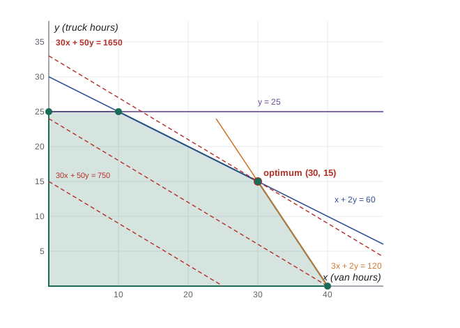

Algorithms for linear programming

George Dantzig's simplex method (1947) walks from vertex to vertex along edges of the polyhedron, always improving the objective, until no neighbouring vertex is better; by convexity that vertex is optimal. In practice simplex is extremely fast and is still the workhorse of commercial solvers. In the worst case, however, it can visit exponentially many vertices: Klee and Minty constructed squashed cubes in 1972 on which the classic pivot rule visits all \(2^n\) corners. Whether some pivot rule always takes polynomially many steps is still open. Spielman and Teng's smoothed analysis (2001) explained the practical success: if the input numbers are perturbed slightly at random, the expected number of steps is polynomial.

The first polynomial-time algorithm was Leonid Khachiyan's ellipsoid method (1979). It keeps an ellipsoid that contains the optimum and repeatedly cuts it in half with a violated constraint, shrinking its volume by a constant factor each time. It is too slow in practice but theoretically powerful, because it needs only a separation oracle: a procedure that, given a point, either confirms it is feasible or returns a violated constraint. That lets it optimize over polyhedra with exponentially many constraints. Narendra Karmarkar's interior-point method (1984) moves through the inside of the polyhedron rather than along its edges and is polynomial and practical; modern solvers offer both simplex and interior-point methods.

# A small exact simplex method (Bland's rule, Fractions) for  max c.x  s.t.  Ax <= b, x >= 0, b >= 0.
# It also returns the dual solution y, read from the final objective row.
from fractions import Fraction as F

def simplex(A, b, c):
    m, n = len(A), len(c)
    T = [[F(v) for v in A[i]] + [F(int(i == j)) for j in range(m)] + [F(b[i])] for i in range(m)]
    z = [F(-v) for v in c] + [F(0)] * m + [F(0)]
    basis = [n + i for i in range(m)]
    while True:
        col = next((j for j in range(n + m) if z[j] < 0), None)      # Bland: lowest index
        if col is None: break
        rows = [(T[i][-1] / T[i][col], basis[i], i) for i in range(m) if T[i][col] > 0]
        if not rows: raise ValueError("unbounded")
        _, _, r = min(rows)
        piv = T[r][col]; T[r] = [v / piv for v in T[r]]
        for i in range(m):
            if i != r and T[i][col]:
                f = T[i][col]; T[i] = [a - f * bb for a, bb in zip(T[i], T[r])]
        f = z[col]; z = [a - f * bb for a, bb in zip(z, T[r])]
        basis[r] = col
    x = [F(0)] * n
    for i, j in enumerate(basis):
        if j < n: x[j] = T[i][-1]
    y = z[n:n + m]                                   # reduced costs of the slacks = dual values
    return z[-1], x, y

A = [[1, 2], [3, 2], [0, 1]]; b = [60, 120, 25]; c = [30, 50]
val, x, y = simplex(A, b, c)
print("primal optimum", val, "at x =", [str(v) for v in x])
print("dual solution  y =", [str(v) for v in y], " dual objective", sum(bi * yi for bi, yi in zip(b, y)))
# complementary slackness: y_i > 0 only where constraint i is tight
for i in range(3):
    lhs = sum(A[i][j] * x[j] for j in range(2))
    print(f"constraint {i + 1}: {lhs} <= {b[i]}  slack {b[i] - lhs}   y_{i + 1} = {y[i]}")
for j in range(2):
    print(f"dual constraint {j + 1}: {sum(A[i][j] * y[i] for i in range(3))} >= {c[j]}")

primal optimum 1650 at x = ['30', '15']
dual solution  y = ['45/2', '5/2', '0']  dual objective 1650
constraint 1: 60 <= 60  slack 0   y_1 = 45/2
constraint 2: 120 <= 120  slack 0   y_2 = 5/2
constraint 3: 15 <= 25  slack 10   y_3 = 0
dual constraint 1: 30 >= 30
dual constraint 2: 50 >= 50

Duality

How could we convince someone that 1650 is the best possible value without showing them the whole feasible region? Combine the constraints with nonnegative multipliers. Multiply the dock constraint \(x + 2y \le 60\) by \(u_1\) and the fuel constraint \(3x + 2y \le 120\) by \(u_2\), and add: \((u_1 + 3u_2)x + (2u_1 + 2u_2)y \le 60u_1 + 120u_2\). If the coefficients on the left are at least 30 and 50 respectively, then because x and y are nonnegative, the objective \(30x + 50y\) is at most the left side, so at most \(60u_1 + 120u_2\). With \(u_1 = 22.5\) and \(u_2 = 2.5\) the coefficients are exactly 30 and 50 and the bound is 1650. The multipliers prove optimality.

Searching for the best such bound is itself a linear program, the dual. For the primal 'maximize \(c^\top x\) subject to \(Ax \le b\), \(x \ge 0\)' the dual is 'minimize \(b^\top y\) subject to \(A^\top y \ge c\), \(y \ge 0\)'. Weak duality. If x is primal feasible and y is dual feasible, then \(c^\top x \le (A^\top y)^\top x = y^\top A x \le y^\top b\). The first inequality uses \(x \ge 0\) and \(A^\top y \ge c\); the second uses \(y \ge 0\) and \(Ax \le b\). Strong duality. If the primal has a finite optimum, so does the dual, and the two optimal values are equal. The proof uses Farkas's lemma, a separating-hyperplane fact about polyhedra, or alternatively the simplex method's final tableau, which contains an optimal dual solution, as the program shows.

Complementary slackness. Feasible x and y are both optimal exactly when (1) every dual variable \(y_i > 0\) has its primal constraint tight, \((Ax)_i = b_i\), and (2) every primal variable \(x_j > 0\) has its dual constraint tight, \((A^\top y)_j = c_j\). This follows by looking at when the two inequalities in the weak duality chain are equalities. Complementary slackness is a practical tool: it turns a guess at a primal solution into a system of equations for the dual, whose feasibility then certifies the guess. In economic terms, \(y_i\) is the shadow price of resource i, the increase in optimal value per extra unit of \(b_i\); a resource with slack has shadow price zero.

Flow and cuts as dual linear programs

Maximum flow is a linear program. One convenient formulation has a variable \(x_P \ge 0\) for each s–t path P, the flow sent along it, and a constraint for each edge e: the total flow on paths through e is at most \(c(e)\). Maximize \(\sum_P x_P\). Its dual has a variable \(y_e \ge 0\) for each edge and a constraint for each path: \(\sum_{e \in P} y_e \ge 1\). Minimize \(\sum_e c(e) y_e\). A 0/1 solution of the dual picks a set of edges that meets every s–t path, which is a cut. So the dual of maximum flow is a fractional minimum cut, and the max-flow min-cut theorem says that this dual always has an integral optimal solution. LP duality explains why flow and cut values meet; the combinatorial proof of lesson 5 explains why the meeting point is an integer cut.

# A small exact simplex method (Bland's rule, Fractions) for  max c.x  s.t.  Ax <= b, x >= 0, b >= 0.
# It also returns the dual solution y, read from the final objective row.
from fractions import Fraction as F

def simplex(A, b, c):
    m, n = len(A), len(c)
    T = [[F(v) for v in A[i]] + [F(int(i == j)) for j in range(m)] + [F(b[i])] for i in range(m)]
    z = [F(-v) for v in c] + [F(0)] * m + [F(0)]
    basis = [n + i for i in range(m)]
    while True:
        col = next((j for j in range(n + m) if z[j] < 0), None)      # Bland: lowest index
        if col is None: break
        rows = [(T[i][-1] / T[i][col], basis[i], i) for i in range(m) if T[i][col] > 0]
        if not rows: raise ValueError("unbounded")
        _, _, r = min(rows)
        piv = T[r][col]; T[r] = [v / piv for v in T[r]]
        for i in range(m):
            if i != r and T[i][col]:
                f = T[i][col]; T[i] = [a - f * bb for a, bb in zip(T[i], T[r])]
        f = z[col]; z = [a - f * bb for a, bb in zip(z, T[r])]
        basis[r] = col
    x = [F(0)] * n
    for i, j in enumerate(basis):
        if j < n: x[j] = T[i][-1]
    y = z[n:n + m]                                   # reduced costs of the slacks = dual values
    return z[-1], x, y


# Maximum flow as a linear program on the diamond network, with path variables:
# one variable per s-t path, one constraint per edge (total flow on paths through e <= c(e)).
edges = {"s-a": 3, "s-b": 2, "a-b": 1, "a-t": 2, "b-t": 3}
paths = [["s-a", "a-t"], ["s-b", "b-t"], ["s-a", "a-b", "b-t"]]
names = list(edges)
A = [[1 if e in p else 0 for p in paths] for e in names]
val, x, y = simplex(A, [edges[e] for e in names], [1] * len(paths))
print("max flow (LP):", val, " path flows", [str(v) for v in x])
print("dual edge weights:", {e: str(v) for e, v in zip(names, y) if v})
print("the dual picks a set of edges meeting every path: a cut of capacity",
      sum(edges[e] * v for e, v in zip(names, y)))

max flow (LP): 5  path flows ['2', '2', '1']
dual edge weights: {'s-a': '1', 's-b': '1'}
the dual picks a set of edges meeting every path: a cut of capacity 5

The path formulation has exponentially many variables in general, which is fine for theory but not for computation; the edge formulation with a variable per edge and conservation constraints has polynomial size. Many polynomial-time problems have LP formulations whose constraint matrices are totally unimodular, meaning every square submatrix has determinant 0, 1 or \(-1\). Then every vertex of the polyhedron is integral whenever b is, and the LP solves the integer problem directly. Incidence matrices of directed graphs and of bipartite graphs have this property, which is another explanation of the integrality theorem for flows and of König's theorem.

Integer programming and relaxations

Requiring some variables to be integers gives an integer linear program (ILP). ILPs can express almost any combinatorial optimization problem: a variable \(x_v \in \{0, 1\}\) for each vertex, with \(x_u + x_v \ge 1\) for each edge, minimizing \(\sum x_v\), is exactly minimum vertex cover. Integer programming is NP-hard (lesson 9), and yet branch-and-bound solvers based on LP relaxations solve large practical instances every day. Dropping the integrality requirement gives the LP relaxation, which can be solved in polynomial time and whose optimum bounds the integer optimum. The ratio between the two in the worst case is the integrality gap. For vertex cover on a triangle, the LP sets every \(x_v = 1/2\) for value 1.5 while the integer optimum is 2.

# A small exact simplex method (Bland's rule, Fractions) for  max c.x  s.t.  Ax <= b, x >= 0, b >= 0.
# It also returns the dual solution y, read from the final objective row.
from fractions import Fraction as F

def simplex(A, b, c):
    m, n = len(A), len(c)
    T = [[F(v) for v in A[i]] + [F(int(i == j)) for j in range(m)] + [F(b[i])] for i in range(m)]
    z = [F(-v) for v in c] + [F(0)] * m + [F(0)]
    basis = [n + i for i in range(m)]
    while True:
        col = next((j for j in range(n + m) if z[j] < 0), None)      # Bland: lowest index
        if col is None: break
        rows = [(T[i][-1] / T[i][col], basis[i], i) for i in range(m) if T[i][col] > 0]
        if not rows: raise ValueError("unbounded")
        _, _, r = min(rows)
        piv = T[r][col]; T[r] = [v / piv for v in T[r]]
        for i in range(m):
            if i != r and T[i][col]:
                f = T[i][col]; T[i] = [a - f * bb for a, bb in zip(T[i], T[r])]
        f = z[col]; z = [a - f * bb for a, bb in zip(z, T[r])]
        basis[r] = col
    x = [F(0)] * n
    for i, j in enumerate(basis):
        if j < n: x[j] = T[i][-1]
    y = z[n:n + m]                                   # reduced costs of the slacks = dual values
    return z[-1], x, y


# Integrality gaps: the fractional matching LP  max sum y_e  s.t.  sum of y_e at each vertex <= 1.
# By LP duality its optimum equals the fractional vertex cover optimum.
from itertools import combinations

def frac_matching(n, E):
    A = [[1 if v in e else 0 for e in E] for v in range(n)]
    val, y, _ = simplex(A, [1] * n, [1] * len(E))
    return val

def integer_matching(E):
    return max(r for r in range(len(E) + 1) for M in combinations(E, r)
               if len({v for e in M for v in e}) == 2 * r)

def integer_cover(n, E):
    return min(k for k in range(n + 1) for C in combinations(range(n), k)
               if all(u in C or v in C for u, v in E))

graphs = {"triangle": (3, [(0, 1), (1, 2), (0, 2)]),
          "5-cycle": (5, [(i, (i + 1) % 5) for i in range(5)]),
          "path of 4": (4, [(0, 1), (1, 2), (2, 3)]),
          "K4": (4, list(combinations(range(4), 2)))}
print(f"{'graph':10s} {'integer matching':>17} {'LP value':>9} {'integer cover':>14}")
for name, (n, E) in graphs.items():
    print(f"{name:10s} {integer_matching(E):17d} {str(frac_matching(n, E)):>9} {integer_cover(n, E):14d}")

graph       integer matching  LP value  integer cover
triangle                   1       3/2              2
5-cycle                    2       5/2              3
path of 4                  2         2              2
K4                         2         2              3

The table shows that for bipartite graphs such as the path, integer matching, the LP and integer vertex cover all agree, as König's theorem predicts. On odd cycles and complete graphs they separate, and the LP value sits between the integer matching and the integer cover. Lesson 10 shows how to round the vertex cover LP to get a cover at most twice the LP value, hence at most twice optimal.

Worked examples