Network flow: Ford–Fulkerson, Edmonds–Karp and max-flow min-cut

Every evening Aspen Valley's trucks carry parcels from the main depot to a regional hub, over a network of roads and transfer points. Each road segment can handle only so many truckloads per night, because of weight restrictions, driver hours and loading docks. How many truckloads can reach the hub, and which roads are the bottleneck? This is the maximum flow problem. It is one of the great success stories of algorithm design: it has a beautiful theory, a simple algorithm with several fast refinements, and an astonishing range of applications, many of which look nothing like flow at first sight. This lesson develops the theory and the algorithms; lesson 6 is devoted to applications. MATH-460 studies the same theorem from the combinatorial side, with Menger's theorem and König's theorem; here the focus is on algorithms and their running times.

Flow networks

A flow network is a directed graph \(G = (V, E)\) with a source s, a sink t and a nonnegative capacity \(c(e)\) on each edge. A flow assigns a value \(f(e)\) to each edge such that (1) \(0 \le f(e) \le c(e)\) for every edge (the capacity constraint), and (2) for every vertex v other than s and t, the flow into v equals the flow out of v (conservation). The value of the flow, \(|f|\), is the net flow out of s, which by conservation equals the net flow into t. The problem is to find a flow of maximum value.

Flow problems were first studied for real transport networks. In 1955 T. E. Harris and F. S. Ross analysed the Soviet rail network for the US Air Force, looking for the cheapest set of lines to cut, in a report declassified only in 1999; Russian work by A. N. Tolstoi on rail transport dates from 1930. Lester Ford and Delbert Fulkerson, at RAND, proved the max-flow min-cut theorem and gave their augmenting-path algorithm in 1956.

Augmenting paths and the residual graph

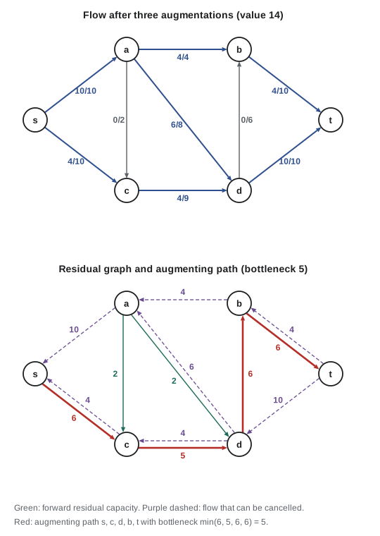
A natural first idea is greedy: find any path from s to t on which every edge has spare capacity, push as much flow as the tightest edge allows, and repeat. This can get stuck at a flow that is not maximum, because an early choice uses an edge that a better solution would leave alone. The fix is to allow later paths to undo earlier decisions. The residual graph \(G_f\) of a flow f has, for each edge \((u, v)\), a forward edge with residual capacity \(c(u, v) - f(u, v)\) when this is positive, and a backward edge \((v, u)\) with residual capacity \(f(u, v)\) when this is positive. Pushing flow along a backward edge cancels flow previously sent forward.

# Why we need the residual graph: augmenting only along original edges can get stuck.
# Diamond network: s->a, s->b, a->b, a->t, b->t, all capacity 1. Maximum flow is 2.
cap = {("s", "a"): 1, ("s", "b"): 1, ("a", "b"): 1, ("a", "t"): 1, ("b", "t"): 1}

def find_path(r, s, t, seen=None):
    seen = seen or {s}
    if s == t: return [t]
    for (u, v), c in sorted(r.items()):
        if u == s and c > 0 and v not in seen:
            seen.add(v)
            rest = find_path(r, v, t, seen)
            if rest: return [s] + rest
    return None

def augment_all(r, use_reverse):
    total = 0
    while True:
        p = find_path(r, "s", "t")
        if not p: return total
        print("   augment along", "-".join(p))
        for u, v in zip(p, p[1:]):
            r[(u, v)] -= 1
            if use_reverse: r[(v, u)] = r.get((v, u), 0) + 1      # undo capacity
        total += 1

order = {("s", "a"): 1, ("a", "b"): 1, ("b", "t"): 1, ("s", "b"): 1, ("a", "t"): 1}
print("greedy, original edges only:")
print("   value", augment_all(dict(order), use_reverse=False))
print("Ford-Fulkerson with residual (reverse) edges:")
print("   value", augment_all(dict(order), use_reverse=True))

greedy, original edges only:
   augment along s-a-b-t
   value 1
Ford-Fulkerson with residual (reverse) edges:
   augment along s-a-b-t
   augment along s-b-a-t
   value 2

An augmenting path is an s–t path in the residual graph. Its bottleneck is the smallest residual capacity on it. Augmenting by the bottleneck b means adding b to the flow on each forward edge of the path and subtracting b on each backward edge. The result is again a flow: capacities are respected by the choice of b, and at each internal vertex of the path the changes on the incoming and outgoing path edges balance. The value increases by b, because the first edge leaves s. The Ford–Fulkerson method starts with the zero flow and augments until no augmenting path remains.

Cuts and the max-flow min-cut theorem

An s–t cut is a partition of V into a set S containing s and its complement \(T = V \setminus S\) containing t. Its capacity \(c(S, T)\) is the total capacity of edges from S to T; edges from T back to S do not count. Lemma (weak duality). For any flow f and any cut \((S, T)\), \(|f| = f(S, T) - f(T, S) \le c(S, T)\), where \(f(S, T)\) is the total flow on edges from S to T. Proof. Sum the conservation equations over all vertices of S: the net flow out of S equals the net flow out of s, which is \(|f|\), because every internal vertex contributes zero. The edges inside S cancel in the sum, leaving the flow on edges leaving S minus the flow on edges entering S. Since \(f \le c\) on edges leaving and \(f \ge 0\) on edges entering, the bound follows.

So every cut gives an upper bound on every flow. The remarkable fact is that the best bound is exact. Theorem (max-flow min-cut). For a flow f the following are equivalent: (1) f is a maximum flow; (2) the residual graph \(G_f\) has no augmenting path; (3) \(|f| = c(S, T)\) for some cut. Proof. (1) implies (2): an augmenting path would give a larger flow. (3) implies (1): by the lemma no flow exceeds \(c(S, T)\), and f achieves it. (2) implies (3): let S be the set of vertices reachable from s in \(G_f\); t is not in S because there is no augmenting path. Every edge \((u, v)\) from S to T must be saturated, \(f(u, v) = c(u, v)\), since otherwise v would be reachable. Every edge \((v, u)\) from T to S must carry zero flow, since otherwise its backward residual edge would make v reachable. Then the lemma's inequality is an equality: \(|f| = c(S, T)\).

The proof gives more than the theorem. When Ford–Fulkerson stops, the set of vertices reachable from s in the residual graph is a minimum cut, found in linear time. And if all capacities are integers, every augmentation adds an integer, so the algorithm ends with an integer maximum flow. This integrality theorem is what makes flow so useful for combinatorial problems: lesson 6 uses it to turn flows into matchings, assignments and schedules.

# Edmonds-Karp (Ford-Fulkerson with shortest augmenting paths found by BFS),
# then the minimum cut read off from the vertices still reachable in the residual graph.
from collections import deque
cap = {("s", "a"): 10, ("s", "c"): 10, ("a", "b"): 4, ("a", "c"): 2, ("a", "d"): 8,
       ("c", "d"): 9, ("d", "b"): 6, ("b", "t"): 10, ("d", "t"): 10}
V = sorted({x for e in cap for x in e})

def max_flow(cap, s, t):
    r = {}
    for (u, v), c in cap.items():
        r[(u, v)] = r.get((u, v), 0) + c; r.setdefault((v, u), 0)
    adj = {v: [w for (x, w) in r if x == v] for v in V}
    value = 0
    while True:
        par = {s: None}; q = deque([s])
        while q and t not in par:
            u = q.popleft()
            for v in adj[u]:
                if r[(u, v)] > 0 and v not in par:
                    par[v] = u; q.append(v)
        if t not in par:
            return value, r, set(par)                  # par now holds the vertices reachable from s
        path, v = [], t
        while par[v] is not None: path.append((par[v], v)); v = par[v]
        b = min(r[e] for e in path)
        for u, v in path: r[(u, v)] -= b; r[(v, u)] += b
        value += b
        print(f"   path {'-'.join([s] + [v for _, v in reversed(path)])}  bottleneck {b}  total {value}")

value, r, S = max_flow(cap, "s", "t")
flow = {e: cap[e] - r[e] for e in cap}
print("maximum flow:", value)
for v in V:
    if v not in "st":
        assert sum(f for (a, b), f in flow.items() if b == v) == sum(f for (a, b), f in flow.items() if a == v)
print("conservation holds at every internal vertex")
cut = [e for e in cap if e[0] in S and e[1] not in S]
print("minimum cut: S =", sorted(S), " edges", cut, " capacity", sum(cap[e] for e in cut))

   path s-a-b-t  bottleneck 4  total 4
   path s-a-d-t  bottleneck 6  total 10
   path s-c-d-t  bottleneck 4  total 14
   path s-c-d-b-t  bottleneck 5  total 19
maximum flow: 19
conservation holds at every internal vertex
minimum cut: S = ['c', 's']  edges [('s', 'a'), ('c', 'd')]  capacity 19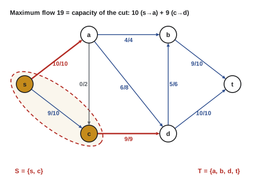

Running time and the choice of path

With integer capacities, each augmentation increases the value by at least 1, so Ford–Fulkerson makes at most \(|f^*|\) augmentations, each taking \(O(m)\) time with a graph search, for \(O(m |f^*|)\) total. That bound is pseudo-polynomial, and it can be reached: on the network below, choosing augmenting paths that zigzag through a middle edge of capacity 1 gains only one unit per augmentation. With irrational capacities a bad choice of paths need not even terminate, and can converge to a value below the maximum.

# Ford-Fulkerson can need as many augmentations as the flow value when paths are chosen badly.
# Network: s->a, s->b, a->t, b->t with capacity C, and a middle edge a->b with capacity 1.
def run(C, choose):
    r = {("s","a"): C, ("s","b"): C, ("a","t"): C, ("b","t"): C, ("a","b"): 1,
         ("a","s"): 0, ("b","s"): 0, ("t","a"): 0, ("t","b"): 0, ("b","a"): 0}
    steps = value = 0
    while True:
        p = choose(r, steps)
        if not p: return value, steps
        b = min(r[(u, v)] for u, v in zip(p, p[1:]))
        for u, v in zip(p, p[1:]): r[(u, v)] -= b; r[(v, u)] += b
        value += b; steps += 1

def zigzag(r, k):                    # alternate s-a-b-t and s-b-a-t while they exist
    for p in ((["s","a","b","t"], ["s","b","a","t"])[k % 2], ["s","a","t"], ["s","b","t"]):
        if all(r[(u, v)] > 0 for u, v in zip(p, p[1:])): return p
    return None

def shortest(r, k):                  # BFS order: two-edge paths first
    for p in (["s","a","t"], ["s","b","t"], ["s","a","b","t"], ["s","b","a","t"]):
        if all(r[(u, v)] > 0 for u, v in zip(p, p[1:])): return p
    return None

for C in (10, 1000, 100000):
    print(f"C = {C:6d}:  bad choices {run(C, zigzag)}   shortest paths {run(C, shortest)}   (value, augmentations)")

C =     10:  bad choices (20, 20)   shortest paths (20, 2)   (value, augmentations)
C =   1000:  bad choices (2000, 2000)   shortest paths (2000, 2)   (value, augmentations)
C = 100000:  bad choices (200000, 200000)   shortest paths (200000, 2)   (value, augmentations)

Edmonds–Karp. Jack Edmonds and Richard Karp proved in 1972 that always augmenting along a shortest path, in number of edges, found by breadth-first search, makes at most \(O(nm)\) augmentations, for \(O(nm^2)\) time overall, independent of the capacities. Yefim Dinitz had published a faster algorithm along the same lines in 1970. The proof rests on two facts. First, the BFS distance \(\delta_f(v)\) from s to any vertex v in the residual graph never decreases. Augmenting along a shortest path removes at least one edge from the residual graph, the bottleneck, and the only edges it can add are reverses of path edges, which go from a vertex at distance \(i + 1\) back to distance i; such edges never create a shorter route. Second, call an edge critical when it is a bottleneck. After \((u, v)\) is critical it disappears from \(G_f\), and it can only reappear after flow is pushed back along \((v, u)\), which requires \((v, u)\) on a shortest path. At the first time \(\delta(v) = \delta(u) + 1\); at the second, \(\delta'(u) = \delta'(v) + 1 \ge \delta(v) + 1 = \delta(u) + 2\). So each time an edge becomes critical again its tail's distance has grown by at least 2, which can happen at most about n/2 times. With \(O(m)\) edges, each critical \(O(n)\) times, and at least one critical edge per augmentation, there are \(O(nm)\) augmentations.

Faster algorithms

Dinitz's algorithm (1970) builds the level graph of BFS distances and finds a blocking flow in it, many shortest paths at once, in \(O(nm)\) time; the distance to t grows with each phase, so there are at most n phases and the total is \(O(n^2 m)\). On unit-capacity graphs it is much faster, which is why it is the standard tool for bipartite matching (lesson 6). Push–relabel algorithms, introduced by Goldberg and Tarjan in 1988, work locally: vertices hold excess flow and push it toward t along edges that go 'downhill' according to height labels, raising labels when stuck. They are often the fastest in practice. In 2022 Chen, Kyng, Liu, Peng, Probst Gutenberg and Sachdeva announced an algorithm that computes maximum flows in \(m^{1 + o(1)}\) time, almost linear, using interior-point methods and dynamic data structures; it settled a question that had been open for decades, though it is not yet a practical tool.

# Max-flow min-cut checked on random networks: the flow value equals the smallest
# capacity over all 2^(n-2) s-t cuts, found here by brute force.
import random
from itertools import combinations
from collections import deque
random.seed(304)

def edmonds_karp(n, cap):
    r = [row[:] for row in cap]; value = 0
    while True:
        par = [-1] * n; par[0] = 0; q = deque([0])
        while q:
            u = q.popleft()
            for v in range(n):
                if r[u][v] > 0 and par[v] < 0: par[v] = u; q.append(v)
        if par[n - 1] < 0: return value
        b, v = float("inf"), n - 1
        while v: b = min(b, r[par[v]][v]); v = par[v]
        v = n - 1
        while v: r[par[v]][v] -= b; r[v][par[v]] += b; v = par[v]
        value += b

def min_cut_brute(n, cap):
    best = float("inf")
    inner = range(1, n - 1)
    for k in range(n - 1):
        for A in combinations(inner, k):
            S = {0, *A}
            best = min(best, sum(cap[u][v] for u in S for v in range(n) if v not in S))
    return best

for trial in range(200):
    n = random.randint(4, 8)
    cap = [[0] * n for _ in range(n)]
    for u in range(n):
        for v in range(n):
            if u != v and random.random() < 0.4: cap[u][v] = random.randint(1, 9)
    assert edmonds_karp(n, cap) == min_cut_brute(n, cap)
print("200 random networks: maximum flow = minimum cut every time")

200 random networks: maximum flow = minimum cut every time

Worked examples