
CMPUT-304 · Lesson 3 of 12 · 31 min
Dynamic programming II: knapsack, intervals and trees
Lesson 2 set out the recipe for dynamic programming and applied it to sequences, where the subproblems are prefixes. This lesson applies the same recipe to three other shapes of subproblem. In the knapsack family, a subproblem is a prefix of the items together with a remaining capacity, which introduces a numeric parameter into the table and with it the idea of pseudo-polynomial time. In interval problems, a subproblem is a contiguous range, and the recurrence chooses where to split it. On trees, a subproblem is a rooted subtree, and the recurrence combines answers from the children. Together with the sequence problems, these patterns cover most of the dynamic programs you will meet in practice.
The 0/1 knapsack problem
An Aspen Valley van has room for 25 kg of extra parcels on a run. Each parcel i has a weight \(w_i\) and a value \(v_i\), the fee earned by delivering it today rather than tomorrow. Which parcels should go in? Formally, given positive integer weights, values and a capacity W, choose a subset \(S\) of items with \(\sum_{i \in S} w_i \le W\) that maximizes \(\sum_{i \in S} v_i\). Each item is taken whole or not at all, hence '0/1'. CMPUT-204 showed that the greedy rule 'take items in order of value per kilogram' is optimal when items can be split (the fractional knapsack) but can fail badly here.
Define \(K[i][w]\) as the largest value achievable using only items 1 to i with capacity w. For the last item there are two choices. If item i is left out, the best is \(K[i-1][w]\). If it is taken, which requires \(w_i \le w\), it contributes \(v_i\) and leaves capacity \(w - w_i\) for the first \(i-1\) items, so the best is \(v_i + K[i-1][w - w_i]\). Therefore \(K[i][w] = \max(K[i-1][w],\ v_i + K[i-1][w - w_i])\), with the second option only when it fits, and \(K[0][w] = 0\). The table has \((n+1)(W+1)\) entries, each computed in constant time.
# 0/1 knapsack for an Aspen Valley van: maximize parcel value within a weight limit.
# K[i][w] = best value using parcels 1..i with capacity w.  Time and space O(nW).
from itertools import combinations

parcels = [("tiles", 12, 40), ("printer", 7, 42), ("bike", 11, 60), ("books", 4, 18),
           ("lamp", 3, 15), ("rug", 9, 37), ("tools", 6, 30), ("monitor", 5, 32)]   # (name, kg, value)
W = 25
n = len(parcels)
K = [[0] * (W + 1) for _ in range(n + 1)]
for i in range(1, n + 1):
    _, wt, val = parcels[i - 1]
    for w in range(W + 1):
        K[i][w] = K[i - 1][w]                                  # skip parcel i
        if wt <= w and K[i - 1][w - wt] + val > K[i][w]:
            K[i][w] = K[i - 1][w - wt] + val                   # take parcel i

chosen, w = [], W
for i in range(n, 0, -1):                                      # trace back
    if K[i][w] != K[i - 1][w]:
        chosen.append(parcels[i - 1][0]); w -= parcels[i - 1][1]
print("best value", K[n][W], "with", sorted(chosen), "weight", W - w, "kg")
print("table cells:", (n + 1) * (W + 1))

best = max(sum(p[2] for p in c) for r in range(n + 1) for c in combinations(parcels, r)
           if sum(p[1] for p in c) <= W)
print("brute force over", 2 ** n, "subsets:", best)

ratio = sorted(parcels, key=lambda p: -p[2] / p[1])            # greedy by value per kg
g, load = 0, 0
for name, wt, val in ratio:
    if load + wt <= W: g += val; load += wt
print("greedy by value per kg:", g)best value 137 with ['bike', 'lamp', 'monitor', 'tools'] weight 25 kg table cells: 234 brute force over 256 subsets: 137 greedy by value per kg: 134
Pseudo-polynomial time and a second table
The running time \(O(nW)\) looks polynomial, but W is a number in the input, written in about \(\log_2 W\) bits. If weights are given to the gram and the capacity is 25,000 g, the table grows a thousandfold. An algorithm whose time is polynomial in the numeric values, but not in the length of the input, is called pseudo-polynomial. Lesson 9 shows that knapsack is NP-complete, so a truly polynomial algorithm is not expected; the pseudo-polynomial one is still extremely useful when the numbers are small.
There is a second dynamic program that swaps the roles of weight and value. Let \(M[v]\) be the smallest total weight of a subset whose value is exactly v. Processing items one at a time and updating values from high to low, so that each item is used at most once, fills this table in \(O(nV)\) time, where V is the sum of all values. The answer is the largest v with \(M[v] \le W\). This version looks no better, but it is the foundation of the knapsack approximation scheme in lesson 10: rounding the values to a coarser scale makes V small while losing only a controlled fraction of the optimum.
# A second knapsack DP indexed by VALUE instead of weight:
# M[v] = minimum weight needed to reach value exactly v.  Time O(n * total value).
parcels = [("tiles", 12, 40), ("printer", 7, 42), ("bike", 11, 60), ("books", 4, 18),
           ("lamp", 3, 15), ("rug", 9, 37), ("tools", 6, 30), ("monitor", 5, 32)]
W = 25
V = sum(p[2] for p in parcels)
INF = float("inf")
M = [0] + [INF] * V
for _, wt, val in parcels:
    for v in range(V, val - 1, -1):          # downward, so each parcel is used at most once
        if M[v - val] + wt < M[v]:
            M[v] = M[v - val] + wt
best = max(v for v in range(V + 1) if M[v] <= W)
print("total value", V, "-> table of", V + 1, "entries")
print("best value within", W, "kg:", best, "(needs", M[best], "kg)")total value 274 -> table of 275 entries best value within 25 kg: 137 (needs 25 kg)
Two relatives deserve mention. In the unbounded knapsack, each item may be taken any number of times, and the recurrence becomes one-dimensional: \(U[w] = \max_i (v_i + U[w - w_i])\) over items that fit. Making change with the fewest coins is the same pattern with a minimum. Subset sum asks whether some subset of numbers adds up to exactly a target T; it is knapsack with values equal to weights and a yes/no question, and it reappears in lesson 9 as a standard NP-complete problem.
Weighted interval scheduling
A driver can take delivery jobs during the day. Job j runs from \(s_j\) to \(f_j\) and pays \(v_j\); two jobs are compatible if they do not overlap. Choose compatible jobs of maximum total pay. When all pays are equal, the greedy 'earliest finish first' rule from CMPUT-204 is optimal. With pays it is not, since one long well-paid job may be worth more than several short ones. Sort the jobs by finish time and let \(p(j)\) be the number of jobs that finish no later than job j starts, so that jobs 1 to \(p(j)\) are exactly those compatible with j among the first \(j-1\). Either job j is in the optimum or it is not: \(\text{OPT}(j) = \max(\text{OPT}(j-1),\ v_j + \text{OPT}(p(j)))\). Sorting and binary searches for the \(p(j)\) values take \(O(n \log n)\) time, and the table takes \(O(n)\) more.
# Weighted interval scheduling: choose non-overlapping delivery jobs of maximum total pay.
# Sort by finish time; p(j) = last job finishing no later than job j starts.
import bisect, random
from itertools import combinations
random.seed(304)

def schedule(jobs):                                  # jobs: (start, finish, pay)
    jobs = sorted(jobs, key=lambda j: j[1])
    finish = [j[1] for j in jobs]
    p = [bisect.bisect_right(finish, s) for s, _, _ in jobs]     # count of jobs compatible before j
    OPT = [0] * (len(jobs) + 1)
    for j in range(1, len(jobs) + 1):
        OPT[j] = max(OPT[j - 1], jobs[j - 1][2] + OPT[p[j - 1]])
    pick, j = [], len(jobs)
    while j:
        if jobs[j - 1][2] + OPT[p[j - 1]] >= OPT[j - 1]:
            pick.append(jobs[j - 1]); j = p[j - 1]
        else:
            j -= 1
    return OPT[-1], pick[::-1]

def brute(jobs):
    best = 0
    for r in range(len(jobs) + 1):
        for c in combinations(sorted(jobs), r):
            if all(c[i][1] <= c[i + 1][0] for i in range(r - 1)):
                best = max(best, sum(x[2] for x in c))
    return best

jobs = [(8, 11, 50), (9, 10, 20), (10, 13, 45), (11, 12, 25), (12, 15, 70), (13, 14, 20), (14, 17, 40)]
val, pick = schedule(jobs)
print("best pay", val, "using", pick)
earliest = sorted(jobs, key=lambda j: j[1]); t, g = 0, 0
for s, f, w in earliest:
    if s >= t: g += w; t = f
print("earliest-finish greedy (optimal only when all pays are equal):", g)
for _ in range(300):
    J = [(s, s + random.randint(1, 5), random.randint(1, 30)) for s in random.sample(range(20), 9)]
    assert schedule(J)[0] == brute(J)
print("300 random instances agree with brute force")best pay 145 using [(8, 11, 50), (11, 12, 25), (12, 15, 70)] earliest-finish greedy (optimal only when all pays are equal): 105 300 random instances agree with brute force
The correctness argument is a clean example of the recipe. Fix an optimal solution for jobs 1 to j. If it does not contain job j, it is a solution for jobs 1 to \(j-1\), and no solution for those can be better, so its value is \(\text{OPT}(j-1)\). If it contains job j, every other chosen job is compatible with j and finishes before j starts, so it lies among jobs 1 to \(p(j)\), and its value is \(v_j\) plus the best value for those, \(\text{OPT}(p(j))\). The maximum of the two cases covers every possibility.
Interval dynamic programming: matrix chains
Multiplying a \(p \times q\) matrix by a \(q \times r\) matrix with the usual algorithm takes \(pqr\) scalar multiplications. Matrix multiplication is associative, so a product \(A_1 A_2 \cdots A_n\) can be parenthesized in many ways, all giving the same result but at very different costs. If \(A_i\) has dimensions \(d_{i-1} \times d_i\), let \(C[i][j]\) be the minimum cost of computing \(A_i \cdots A_j\). The last multiplication splits the range at some k, multiplying the result of \(A_i \cdots A_k\) by that of \(A_{k+1} \cdots A_j\), at cost \(d_{i-1} d_k d_j\). Hence \(C[i][j] = \min_{i \le k < j} (C[i][k] + C[k+1][j] + d_{i-1} d_k d_j)\), with \(C[i][i] = 0\). There are \(O(n^2)\) intervals, each taking \(O(n)\) time, for \(O(n^3)\) overall. The evaluation order is by interval length, since each interval depends only on shorter ones.
# Interval DP: the cheapest order to multiply a chain of matrices.
# C[i][j] = min over i <= k < j of C[i][k] + C[k+1][j] + d[i-1] d[k] d[j].  O(n^3) time.
def chain(d):
    n = len(d) - 1
    C = [[0] * (n + 1) for _ in range(n + 1)]
    S = [[0] * (n + 1) for _ in range(n + 1)]
    for length in range(2, n + 1):                      # solve shorter intervals first
        for i in range(1, n - length + 2):
            j = i + length - 1
            C[i][j] = float("inf")
            for k in range(i, j):
                c = C[i][k] + C[k + 1][j] + d[i - 1] * d[k] * d[j]
                if c < C[i][j]: C[i][j], S[i][j] = c, k
    def paren(i, j):
        return f"A{i}" if i == j else "(" + paren(i, S[i][j]) + " " + paren(S[i][j] + 1, j) + ")"
    return C[1][n], paren(1, n)

d = [30, 35, 15, 5, 10, 20, 25]          # A1 is 30x35, A2 is 35x15, ..., A6 is 20x25
cost, order = chain(d)
print("best:", cost, "scalar multiplications with", order)
left = sum(d[0] * d[k] * d[k + 1] for k in range(1, len(d) - 1))
print("left to right:", left)best: 15125 scalar multiplications with ((A1 (A2 A3)) ((A4 A5) A6)) left to right: 40500
The same split-the-interval pattern solves optimal binary search trees, where frequently searched keys should sit near the root; parsing a sentence with a context-free grammar (the CYK algorithm of CMPUT-474); RNA secondary structure prediction, where bases pair up without crossing; and polygon triangulation. Whenever the natural subproblem is 'the best way to handle items i through j', try an interval DP.
Dynamic programming on trees
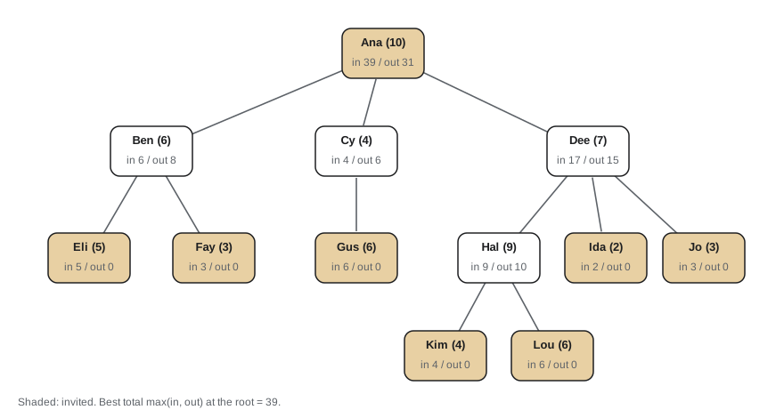
Many problems that are hard on general graphs become easy on trees, because removing a vertex splits a tree into independent pieces. Consider the maximum-weight independent set: choose vertices, no two adjacent, of maximum total weight. On general graphs it is NP-hard (lesson 9). On a tree, root it anywhere and compute two numbers for each vertex v: \(\text{in}(v)\), the best weight in v's subtree when v is chosen, and \(\text{out}(v)\), the best when it is not. If v is chosen, none of its children can be, so \(\text{in}(v) = w_v + \sum_c \text{out}(c)\). If v is not chosen, each child's subtree is free to do its best: \(\text{out}(v) = \sum_c \max(\text{in}(c), \text{out}(c))\). Processing vertices children-first (a post-order) computes everything in \(O(n)\) time.
# Maximum-weight independent set on a tree: invite employees to a party so that nobody
# attends with their direct supervisor, maximizing total "fun" score.
# in[v] = best in v's subtree with v invited; out[v] = best with v not invited.
from itertools import combinations
boss = {"Ana": None, "Ben": "Ana", "Cy": "Ana", "Dee": "Ana", "Eli": "Ben", "Fay": "Ben",
        "Gus": "Cy", "Hal": "Dee", "Ida": "Dee", "Jo": "Dee", "Kim": "Hal", "Lou": "Hal"}
fun = {"Ana": 10, "Ben": 6, "Cy": 4, "Dee": 7, "Eli": 5, "Fay": 3, "Gus": 6,
       "Hal": 9, "Ida": 2, "Jo": 3, "Kim": 4, "Lou": 6}
kids = {v: [c for c, b in boss.items() if b == v] for v in boss}

order, stack = [], ["Ana"]                    # iterative DFS, then process children first
while stack:
    v = stack.pop(); order.append(v); stack.extend(kids[v])
IN, OUT = {}, {}
for v in reversed(order):
    IN[v] = fun[v] + sum(OUT[c] for c in kids[v])
    OUT[v] = sum(max(IN[c], OUT[c]) for c in kids[v])

guests, todo = [], [("Ana", False)]           # recover: (vertex, parent invited?)
while todo:
    v, parent_in = todo.pop()
    take = not parent_in and IN[v] >= OUT[v]
    if take: guests.append(v)
    todo.extend((c, take) for c in kids[v])
print("best fun:", max(IN["Ana"], OUT["Ana"]), "guests:", sorted(guests))

people = list(boss)
best = max(sum(fun[x] for x in S) for r in range(len(people) + 1) for S in combinations(people, r)
           if all(boss[x] not in S for x in S))
print("brute force over", 2 ** len(people), "subsets:", best)best fun: 39 guests: ['Ana', 'Eli', 'Fay', 'Gus', 'Ida', 'Jo', 'Kim', 'Lou'] brute force over 4096 subsets: 39
The two-number trick generalizes. For a vertex cover on a tree, a chosen vertex covers its child edges and an unchosen vertex forces all its children to be chosen. For dominating sets three states are needed: chosen, not chosen but dominated by a child, or not chosen and still waiting for the parent. More broadly, graphs that are 'tree-like', in the precise sense of having small treewidth, admit dynamic programs over a tree decomposition whose running time is exponential only in the width. Lesson 12 returns to this idea as one way of coping with NP-hard problems.
Worked examples
Worked problem
A knapsack table by hand
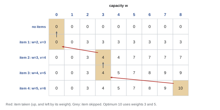
Items with (weight, value) = (2, 3), (3, 4), (4, 5), (5, 6) and capacity 8. Find the optimum.
Show solution
- Row 1 (item of weight 2): value 3 for every capacity at least 2.
- Row 2 adds (3, 4): capacities 5 and up can hold both, value 7.
- Row 3 adds (4, 5): capacity 7 gives 4 + 5 = 9 using weights 3 and 4; capacity 8 still gives 9.
- Row 4 adds (5, 6): capacity 8 can take weights 3 and 5 for 4 + 6 = 10, beating 9.
Answer: Value 10, taking the items of weight 3 and 5.
Worked problem
Computing p(j)
Jobs sorted by finish time: [1, 4), [3, 5), [0, 6), [4, 7), [3, 9), [5, 9), [6, 10), [8, 11). Find p(j) for each.
Show solution
- p(j) counts jobs that finish at or before job j starts.
- Starts 1, 3, 0: no job finishes by then, so p = 0, 0, 0.
- Job [4, 7): job [1, 4) finishes at 4, so p = 1. Job [3, 9): p = 0.
- Job [5, 9): jobs ending at 4 and 5 qualify, p = 2. Job [6, 10): ending at 4, 5, 6, p = 3. Job [8, 11): ending at 4, 5, 6, 7, p = 4.
Answer: p = 0, 0, 0, 1, 0, 2, 3, 4.
Worked problem
Vertex cover on a path
Find a minimum vertex cover of the path a - b - c - d - e using tree DP rooted at a.
Show solution
- Let in(v) and out(v) be the smallest covers of v's subtree with and without v.
- Leaf e: in = 1, out = 0. At d: in = 1 + min(1, 0) = 1, out = in(e) = 1.
- At c: in = 1 + min(1, 1) = 2, out = in(d) = 1. At b: in = 1 + min(2, 1) = 2, out = in(c) = 2.
- At a: in = 1 + min(2, 2) = 3, out = in(b) = 2.
Answer: The minimum cover has size 2, for example {b, d}.
Common mistakes
MistakeCall the O(nW) knapsack algorithm polynomial.
InsteadIt is pseudo-polynomial: W is a number, exponential in its bit length.
MistakeUpdate a one-dimensional 0/1 knapsack table from low capacities to high.
InsteadGo from high to low, otherwise an item can be used more than once.
MistakeUse the greedy earliest-finish rule when jobs have different pays.
InsteadIt is optimal only for equal pays; use the DP with p(j).
MistakeFill an interval DP row by row.
InsteadFill by increasing interval length, since each interval depends on shorter ones.
MistakeApply tree DP to a graph with cycles.
InsteadIt relies on subtrees being independent; for general graphs use tree decompositions or other methods.
Summary and key terms
- 0/1 knapsack: K[i][w] = max(K[i-1][w], v_i + K[i-1][w - w_i]), O(nW) time, pseudo-polynomial.
- A value-indexed DP runs in O(nV) time and underlies the knapsack approximation scheme.
- Weighted interval scheduling: sort by finish time, OPT(j) = max(OPT(j-1), v_j + OPT(p(j))), O(n log n).
- Interval DP splits a range i..j at every k and fills by increasing length; matrix chains take O(n^3).
- Tree DP computes a few values per vertex from its children; maximum-weight independent set on a tree takes O(n).
- 0/1 knapsack
- Choose whole items of maximum value within a weight limit.
- Unbounded knapsack
- Knapsack where each item may be used any number of times.
- Subset sum
- Decide whether some subset of numbers sums exactly to a target.
- Weighted interval scheduling
- Choose non-overlapping intervals of maximum total weight.
- Interval DP
- A DP whose subproblems are contiguous ranges, split at every possible point.
- Independent set
- A set of vertices with no two adjacent.
- Treewidth
- A measure of how close a graph is to a tree; small treewidth enables DP over a tree decomposition.
Practice problems
Work each problem on paper first, then reveal the answer to check.
Give a 0/1 knapsack instance where greedy by value per weight fails.
Show answer
Capacity 10; items (6, 7) and two of (5, 5): greedy takes the 6 kg item for 7, while the two 5 kg items give 10.
Write the unbounded knapsack recurrence.
Show answer
\(U[w] = \max(0, \max_{i: w_i \le w} (v_i + U[w - w_i]))\).
How many entries does the knapsack table have for 100 items and W = 10,000?
Show answer
101 times 10,001, about a million.
In weighted interval scheduling, why sort by finish time?
Show answer
So that the jobs compatible with j among the earlier ones form a prefix 1..p(j).
Two matrices: A is 10 x 100 and B is 100 x 5. What does AB cost?
Show answer
10 x 100 x 5 = 5000 scalar multiplications.
What order does an interval DP use?
Show answer
Increasing interval length.
For a star whose middle vertex has weight 10 and whose five leaves have weight 3, what is the maximum-weight independent set?
Show answer
The five leaves, weight 15.
Why does the tree DP not work directly on a cycle?
Show answer
Removing a vertex does not split a cycle into independent parts; fix one vertex in or out and solve the remaining path twice.
Lesson quiz · 5 questions
Score 60% or more to complete this lesson.
Create a free account to save your progress, take quizzes and earn a certificate.