Dynamic programming I: principles, memoization and sequences

Divide and conquer, from CMPUT-204, splits a problem into independent subproblems, solves them recursively and combines the answers. Many problems split naturally into subproblems that are not independent: the same smaller question comes up again and again along different branches of the recursion. A plain recursive algorithm then repeats an enormous amount of work. Dynamic programming removes the repetition by solving each distinct subproblem once and storing its answer. The idea is simple, but applying it well takes practice, because the hard part is choosing the right subproblems. This lesson develops the method on small examples and then on sequence problems: the longest common subsequence, edit distance and the longest increasing subsequence.

Richard Bellman developed the method at the RAND Corporation in the early 1950s for multistage decision problems, and set it out in his 1957 book Dynamic Programming. 'Programming' meant planning, as in 'linear programming', not writing code. Bellman later wrote that he chose the word 'dynamic' partly because it sounded impressive and was hard to object to. Today dynamic programming runs inside spelling checkers, DNA sequence aligners, speech recognizers, file comparison tools such as diff, route planners and compilers.

Overlapping subproblems: a first example

The Fibonacci numbers satisfy \(F_0 = 0\), \(F_1 = 1\) and \(F_n = F_{n-1} + F_{n-2}\). A recursive function that follows the definition literally calls itself on \(n-1\) and \(n-2\); the call on \(n-1\) calls \(n-2\) again, and so on. The number of calls satisfies \(C(n) = C(n-1) + C(n-2) + 1\), which grows like \(\varphi^n\) with \(\varphi \approx 1.618\), even though there are only \(n+1\) distinct subproblems. There are two standard remedies. Memoization keeps the recursive structure but records each answer in a table the first time it is computed, and looks it up afterwards. Tabulation, or bottom-up dynamic programming, fills the table in an order where every subproblem is solved after the subproblems it depends on, with no recursion at all.

# Three ways to compute Fibonacci numbers, counting the work each one does.
from functools import lru_cache

calls = 0
def fib_naive(n):
    global calls
    calls += 1
    return n if n < 2 else fib_naive(n - 1) + fib_naive(n - 2)

memo_calls = 0
@lru_cache(maxsize=None)
def fib_memo(n):
    global memo_calls
    memo_calls += 1                     # counts only calls that actually compute
    return n if n < 2 else fib_memo(n - 1) + fib_memo(n - 2)

def fib_table(n):
    a, b = 0, 1                         # F(i), F(i+1); only two values are ever needed
    for _ in range(n):
        a, b = b, a + b
    return a

print(" n   F(n)        naive calls   memo computations   table steps")
for n in (10, 20, 25, 30):
    calls = 0; memo_calls = 0; fib_memo.cache_clear()
    v = fib_naive(n); m = fib_memo(n)
    assert v == m == fib_table(n)
    print(f"{n:2d}   {v:9d}   {calls:11d}   {memo_calls:17d}   {n:11d}")
print("F(300) has", len(str(fib_table(300))), "digits; the table method computes it instantly")

 n   F(n)        naive calls   memo computations   table steps
10          55           177                  11            10
20        6765         21891                  21            20
25       75025        242785                  26            25
30      832040       2692537                  31            30
F(300) has 63 digits; the table method computes it instantly

Both remedies do \(O(n)\) additions. Memoization is often easier to write, because it follows the recurrence directly and only computes subproblems that are actually needed. Tabulation avoids recursion depth limits and function-call overhead, and makes it easy to see which table entries can be discarded: here only the last two values are ever needed, so the space drops to \(O(1)\).

The recipe

Most dynamic programming algorithms are designed in the same five steps. (1) Define the subproblems. Say precisely, in words, what each table entry means, for example '\(L[i][j]\) is the length of a longest common subsequence of the first i characters of x and the first j characters of y'. (2) Write the recurrence. Express each entry in terms of smaller entries by considering the possible choices for one decision, usually the last or the first. (3) Give the base cases. (4) Choose an evaluation order in which dependencies are computed first. (5) Recover the solution, not just its value, by storing which choice achieved the optimum, or by retracing the recurrence from the final entry. The running time is the number of subproblems times the time to evaluate one entry.

Two properties make the recipe work. Optimal substructure means that an optimal solution to a problem contains optimal solutions to its subproblems, so that combining the best sub-answers gives the best answer. Overlapping subproblems means that the number of distinct subproblems is small, typically polynomial, even though a naive recursion visits them exponentially often. Optimal substructure is not automatic. A shortest path from s to t that passes through v consists of shortest paths from s to v and from v to t. But a longest simple path does not have this property: the longest simple paths from s to v and from v to t can share vertices, and then their union is not simple. That failure is a first hint of why lesson 1 listed longest path as hard.

Correctness proofs

A dynamic programming algorithm is proved correct by strong induction over the evaluation order. The induction hypothesis is that every entry computed before the current one is correct, meaning that it equals the value promised by the definition in step 1. The inductive step argues that the recurrence considers every possible way an optimal solution can begin or end, and that for each way the best completion is given by an entry that has already been computed. Both directions are needed: the value computed is achievable, because each option corresponds to a real solution, and nothing better exists, because every solution falls into one of the options. Writing the definition of the table entry clearly in words is what makes these proofs short.

Counting with dynamic programming

Dynamic programming also counts. Suppose an Aspen Valley van leaves the depot at the south-west corner of a street grid and must reach a customer seven blocks east and five blocks north, always driving east or north. Without obstacles the number of routes is \(\binom{12}{7} = 792\), since a route is a choice of which 7 of the 12 blocks go east. With some intersections closed for road works there is no simple formula, but the number of routes to intersection \((i, j)\) is the number to \((i-1, j)\) plus the number to \((i, j-1)\), and zero at a closed intersection.

# Counting delivery routes on a street grid that only go east or north,
# avoiding blocked intersections (road works). N[i][j] = N[i-1][j] + N[i][j-1].
W, H = 7, 5                                     # blocks east and north
blocked = {(2, 1), (3, 3), (5, 2)}

N = [[0] * (H + 1) for _ in range(W + 1)]
for i in range(W + 1):
    for j in range(H + 1):
        if (i, j) in blocked:
            N[i][j] = 0
        elif i == 0 and j == 0:
            N[i][j] = 1
        else:
            N[i][j] = (N[i - 1][j] if i else 0) + (N[i][j - 1] if j else 0)

for j in range(H, -1, -1):                       # print with north at the top
    print(" ".join(f"{N[i][j]:4d}" if (i, j) not in blocked else "   X" for i in range(W + 1)))
from math import comb
print("routes with no road works:", comb(W + H, W), "  with road works:", N[W][H])

   1    6   18   30   48   72  106  159
   1    5   12   12   18   24   34   53
   1    4    7    X    6    6   10   19
   1    3    3    4    6    X    4    9
   1    2    X    1    2    3    4    5
   1    1    1    1    1    1    1    1
routes with no road works: 792   with road works: 159

Longest common subsequence

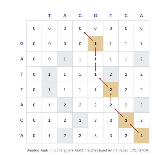
A subsequence of a string is obtained by deleting zero or more characters without reordering the rest. Given strings \(x = x_1 \dots x_m\) and \(y = y_1 \dots y_n\), the longest common subsequence (LCS) problem asks for a longest string that is a subsequence of both. LCS measures similarity: version control tools such as diff compute it line by line to show which lines changed, and biologists use related measures to compare genes. Let \(L[i][j]\) be the length of an LCS of the prefixes \(x_1 \dots x_i\) and \(y_1 \dots y_j\). Consider the last characters. If \(x_i = y_j\), some LCS of the prefixes ends with that character, so \(L[i][j] = L[i-1][j-1] + 1\). Otherwise an LCS cannot end with both of them, so one of them can be dropped: \(L[i][j] = \max(L[i-1][j], L[i][j-1])\). The base cases are \(L[i][0] = L[0][j] = 0\).

Claim. If \(x_i = y_j\) then \(L[i][j] = L[i-1][j-1] + 1\). Proof. Appending the common character to an LCS of the shorter prefixes gives a common subsequence of length \(L[i-1][j-1] + 1\), so \(L[i][j]\) is at least that. For the other direction, take an LCS z of the two prefixes, viewed as a set of matched pairs of positions that do not cross. If neither \(x_i\) nor \(y_j\) is matched, adding the pair \((x_i, y_j)\) gives a longer common subsequence, which is impossible. If only \(x_i\) is matched, it is matched to some \(y_{j'}\) with \(j' < j\), and since \(x_i\) is the last character of its prefix, \(y_{j'}\) is the last matched character of y; rematching \(x_i\) to \(y_j\) keeps the pairs non-crossing and the length the same. The case where only \(y_j\) is matched is symmetric. If both are matched, they must be matched to each other, since otherwise the two pairs would cross. In every case we get an LCS that matches \(x_i\) with \(y_j\), and removing that pair leaves a common subsequence of the shorter prefixes, of length at most \(L[i-1][j-1]\). The table has \((m+1)(n+1)\) entries, each computed in constant time, so the algorithm runs in \(O(mn)\) time.

Edit distance

The edit distance (or Levenshtein distance, after Vladimir Levenshtein's 1965 paper) between two strings is the minimum number of single-character insertions, deletions and substitutions that turn one into the other. Spelling checkers suggest dictionary words at small edit distance from a misspelling, and genome aligners use weighted variants. Let \(D[i][j]\) be the edit distance between the prefixes of length i and j. An optimal sequence of edits can be pictured as an alignment in which each column pairs a character of x with a character of y, or with a gap. Look at the last column: either \(x_i\) is deleted, costing \(1 + D[i-1][j]\); or \(y_j\) is inserted, costing \(1 + D[i][j-1]\); or \(x_i\) is aligned with \(y_j\), costing \(D[i-1][j-1]\) plus 1 if they differ. So \(D[i][j]\) is the minimum of these three, with \(D[i][0] = i\) and \(D[0][j] = j\). Wagner and Fischer published this algorithm in 1974, and it had been found independently several times before.

# Longest common subsequence and edit distance, with the solutions recovered by tracing back.
def lcs(x, y):
    m, n = len(x), len(y)
    L = [[0] * (n + 1) for _ in range(m + 1)]
    for i in range(1, m + 1):
        for j in range(1, n + 1):
            L[i][j] = L[i-1][j-1] + 1 if x[i-1] == y[j-1] else max(L[i-1][j], L[i][j-1])
    out, i, j = [], m, n                        # trace back from the bottom-right corner
    while i and j:
        if x[i-1] == y[j-1]: out.append(x[i-1]); i -= 1; j -= 1
        elif L[i-1][j] >= L[i][j-1]: i -= 1
        else: j -= 1
    return L[m][n], "".join(reversed(out))

def edit(x, y):
    m, n = len(x), len(y)
    D = [[0] * (n + 1) for _ in range(m + 1)]
    for i in range(m + 1): D[i][0] = i
    for j in range(n + 1): D[0][j] = j
    for i in range(1, m + 1):
        for j in range(1, n + 1):
            D[i][j] = min(D[i-1][j] + 1,                        # delete x[i-1]
                          D[i][j-1] + 1,                        # insert y[j-1]
                          D[i-1][j-1] + (x[i-1] != y[j-1]))     # match or substitute
    top, bot, i, j = [], [], m, n
    while i or j:
        if i and j and D[i][j] == D[i-1][j-1] + (x[i-1] != y[j-1]):
            top.append(x[i-1]); bot.append(y[j-1]); i -= 1; j -= 1
        elif i and D[i][j] == D[i-1][j] + 1:
            top.append(x[i-1]); bot.append("-"); i -= 1
        else:
            top.append("-"); bot.append(y[j-1]); j -= 1
    return D[m][n], "".join(reversed(top)), "".join(reversed(bot))

for x, y in (("GATTACA", "TACGTCA"), ("SNOWY", "SUNNY"), ("dynamic", "dynamite")):
    k, s = lcs(x, y)
    d, a, b = edit(x, y)
    print(f"{x} / {y}: LCS length {k} ({s}), edit distance {d}")
    print("   ", a); print("   ", b)

GATTACA / TACGTCA: LCS length 4 (GTCA), edit distance 4
    GATTACA
    TACGTCA
SNOWY / SUNNY: LCS length 3 (SNY), edit distance 3
    SNOWY
    SUNNY
dynamic / dynamite: LCS length 6 (dynami), edit distance 2
    dynami-c
    dynamite

The traceback prefers diagonal moves, so the alignment of SNOWY and SUNNY shows three substitutions; other alignments with the same cost use gaps instead. Several optimal alignments often exist, and the traceback picks one according to the order in which it tests the cases. The LCS and the edit distance are related but not identical: if only insertions and deletions were allowed, the distance would be \(m + n - 2\,\text{LCS}(x, y)\), which for dynamic and dynamite is 7 + 8 - 12 = 3, while substitutions bring it down to 2.

Longest increasing subsequence

Given numbers \(a_1, \dots, a_n\), find a longest subsequence that is strictly increasing. Let \(\ell(j)\) be the length of a longest increasing subsequence that ends at position j. It is 1 plus the largest \(\ell(i)\) over \(i < j\) with \(a_i < a_j\), or just 1 if there is no such i. The answer is the largest \(\ell(j)\). This takes \(O(n^2)\) time. Choosing the subproblem 'ending exactly at j' rather than 'within the first j elements' is the key move: the second version does not have a simple recurrence because we would not know the last value used.

A faster method keeps, for each length k, the smallest possible last element of an increasing subsequence of length k. These tails are themselves increasing, so each new element finds its place by binary search, giving \(O(n \log n)\) time. The idea is related to the card game patience, and the analysis of its pile structure connects to deep results in combinatorics. Testing a clever algorithm against a slow, obviously correct one on many random inputs is a habit worth keeping: it catches most bugs in a few seconds.

# Longest increasing subsequence: the O(n^2) DP, the O(n log n) method, and a brute-force check.
import bisect, random
from itertools import combinations
random.seed(304)

def lis_quadratic(a):
    n = len(a); best = [1] * n; prev = [-1] * n
    for j in range(n):
        for i in range(j):
            if a[i] < a[j] and best[i] + 1 > best[j]:
                best[j], prev[j] = best[i] + 1, i
    j = max(range(n), key=best.__getitem__); seq = []
    while j != -1: seq.append(a[j]); j = prev[j]
    return seq[::-1]

def lis_fast(a):
    tails, tail_idx, prev = [], [], [-1] * len(a)    # tails[k] = smallest tail of an increasing run of length k+1
    for j, x in enumerate(a):
        k = bisect.bisect_left(tails, x)
        if k == len(tails): tails.append(x); tail_idx.append(j)
        else: tails[k] = x; tail_idx[k] = j
        prev[j] = tail_idx[k - 1] if k else -1
    j, seq = tail_idx[-1], []
    while j != -1: seq.append(a[j]); j = prev[j]
    return seq[::-1]

def lis_brute(a):
    for r in range(len(a), 0, -1):
        for c in combinations(a, r):
            if all(c[i] < c[i + 1] for i in range(r - 1)): return r

a = [random.randint(1, 50) for _ in range(16)]
print("sequence:", a)
print("O(n^2) DP:   ", lis_quadratic(a))
print("O(n log n):  ", lis_fast(a))
print("brute force length:", lis_brute(a))
for trial in range(200):                          # random tests against brute force
    b = [random.randint(1, 20) for _ in range(random.randint(1, 11))]
    assert len(lis_quadratic(b)) == len(lis_fast(b)) == lis_brute(b)
print("200 random tests agree")

sequence: [9, 14, 28, 33, 29, 4, 15, 43, 47, 20, 16, 38, 48, 15, 49, 4]
O(n^2) DP:    [9, 14, 28, 33, 43, 47, 48, 49]
O(n log n):   [9, 14, 28, 29, 43, 47, 48, 49]
brute force length: 8
200 random tests agree

Saving space

The edit-distance recurrence only looks at the current row and the one above it, so the full table is not needed to compute the value: two rows suffice, using \(O(\min(m, n))\) space. Recovering an optimal alignment seems to need the whole table for the traceback, but Hirschberg showed in 1975 how to recover it in linear space by divide and conquer: compute the middle row's values from both ends, find where an optimal alignment crosses the middle row, and recurse on the two halves. The total time stays \(O(mn)\). For long DNA sequences this is the difference between needing gigabytes and needing kilobytes.

# Edit distance in O(min(m, n)) space by keeping only two rows of the table.
def edit_two_rows(x, y):
    if len(y) > len(x): x, y = y, x               # make y the shorter string
    prev = list(range(len(y) + 1))
    for i in range(1, len(x) + 1):
        cur = [i] + [0] * len(y)
        for j in range(1, len(y) + 1):
            cur[j] = min(prev[j] + 1, cur[j - 1] + 1, prev[j - 1] + (x[i - 1] != y[j - 1]))
        prev = cur
    return prev[-1]

import random
random.seed(304)
A = "".join(random.choice("ACGT") for _ in range(3000))
B = list(A)
for _ in range(150):                               # mutate: 150 random substitutions
    k = random.randrange(len(B)); B[k] = random.choice("ACGT")
B = "".join(B[:1000] + B[1040:])                   # and delete a block of 40
d = edit_two_rows(A, B)
print("lengths", len(A), len(B), " edit distance", d)
print("full table cells:", (len(A) + 1) * (len(B) + 1), "  two-row cells:", 2 * (len(B) + 1))

lengths 3000 2960  edit distance 148
full table cells: 8885961   two-row cells: 5922

Worked examples