Chemical equilibrium in analysis: activity and systematic treatment

In CHEM-102 you solved equilibrium problems with ICE tables, concentrations in place of activities, and approximations such as neglecting the x in 0.10 − x. Those methods work well for teaching and for many practical problems, but analytical chemists need more. Real samples contain salts at significant concentrations, which change the effective concentrations of ions. Some problems involve several simultaneous equilibria, such as a precipitate whose anion is also a weak base, where an ICE table quickly becomes unmanageable. And sometimes the usual approximations fail outright, as in the classic puzzle of the pH of 10⁻⁸ M HCl. This lesson introduces the two tools that handle all of these cases: activity coefficients and the systematic treatment of equilibrium.

Why concentration is not enough

An ion in solution is surrounded by an ionic atmosphere: a slight excess of oppositely charged ions attracted to it and a slight deficit of like-charged ions. This atmosphere partly shields the ion's charge, lowering its tendency to react with other ions. As a result, an ion behaves as if its concentration were lower than it really is, and the effect grows with the total concentration and charge of all the ions present.

A striking demonstration is the solubility of a sparingly soluble salt in a solution of an unrelated, inert salt. Calcium sulfate is about 1.5 times more soluble in 0.10 M potassium nitrate than in pure water, even though neither K⁺ nor NO₃⁻ is involved in the equilibrium. The ionic atmospheres of the dissolved ions stabilize Ca²⁺ and SO₄²⁻ in solution, so more salt must dissolve to reach equilibrium. This salt effect, which some textbooks call salting in, is the opposite of the common-ion effect.

Ionic strength

The extent of the shielding depends on the ionic strength, μ (also written I), a measure of the total concentration of ions in which each ion is weighted by the square of its charge:

The square of the charge means that doubly and triply charged ions contribute heavily. For a 1:1 electrolyte such as NaCl, μ equals the concentration; for a 2:1 electrolyte such as CaCl₂, μ is three times the concentration; and for a 2:2 electrolyte such as MgSO₄, μ is four times the concentration.

Fresh waters typically have ionic strengths of 0.001 to 0.01 M, blood about 0.16 M, and seawater about 0.7 M. Many groundwaters on the Canadian Prairies and in the upper Midwest of the United States are rich in calcium, magnesium and sulfate and have ionic strengths of 0.01 to 0.05 M, high enough that activity corrections matter for accurate equilibrium calculations.

Activity and activity coefficients

The activity of a species, A_C, is its effective concentration, related to its molar concentration by the activity coefficient γ_C:

Thermodynamically correct equilibrium constants are written in terms of activities. For the solubility of calcium sulfate, for example,

In very dilute solutions γ approaches 1 and activities equal concentrations, which is why the simpler CHEM-102 treatment works there. As ionic strength rises, γ falls below 1, so the product of concentrations must be larger to give the same K. That is the salt effect.

Peter Debye and Erich Hückel derived the activity coefficient of an ion from the electrostatics of the ionic atmosphere in 1923. The extended Debye–Hückel equation, valid up to about μ = 0.1 M, is

for water at 25 °C, where z is the ion's charge and α is its effective hydrated radius in picometres (about 900 pm for H⁺, 600 pm for Ca²⁺ and Mg²⁺, 400 pm for SO₄²⁻ and 300 pm for K⁺ and Cl⁻). In the limit of very low μ the denominator approaches 1, giving the Debye–Hückel limiting law, log γ = −0.51z²√μ.

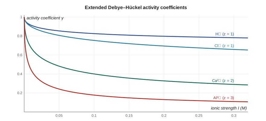
Three trends follow from the equation and the figure. First, γ decreases as ionic strength increases. Second, the effect grows with the square of the charge, so at μ = 0.1 M a singly charged ion has γ ≈ 0.78, a doubly charged ion γ ≈ 0.40 and a triply charged ion γ ≈ 0.18 (typical values). Third, small, highly hydrated ions such as H⁺ and Li⁺ have larger effective radii and are shielded less, so their γ values are closer to 1. Neutral molecules have γ ≈ 1 at moderate ionic strength. Above about 0.5 M, activity coefficients pass through a minimum and rise again, and more elaborate models, such as the Davies equation or Pitzer's equations, are needed.

import math

ALPHA = {'H': 900, 'Ca': 600, 'SO4': 400, 'K': 300, 'NO3': 300, 'Cl': 300}

def gamma(z, mu, a_pm):
    s = math.sqrt(mu)
    return 10 ** (-0.51 * z * z * s / (1 + a_pm * s / 305))

def caso4_solubility(salt=0.0, Ksp=2.4e-5):
    s = math.sqrt(Ksp)
    for _ in range(100):                       # iterate: solubility -> ionic strength -> gammas
        mu = 0.5 * (4 * s + 4 * s) + salt      # Ca2+ and SO4 2- (z^2 = 4) plus a 1:1 salt
        g = gamma(2, mu, ALPHA['Ca']) * gamma(2, mu, ALPHA['SO4'])
        s_new = math.sqrt(Ksp / g)
        if abs(s_new - s) < 1e-12: break
        s = s_new
    return s, mu, g

for salt in (0.0, 0.01, 0.05, 0.10):
    s, mu, g = caso4_solubility(salt)
    print(f"KNO3 {salt:.2f} M: mu = {mu:.4f} M, gamma product = {g:.3f}, solubility = {s * 1000:.2f} mM")
print(f"no activity correction: {math.sqrt(2.4e-5) * 1000:.2f} mM")

KNO3 0.00 M: mu = 0.0398 M, gamma product = 0.243, solubility = 9.94 mM
KNO3 0.01 M: mu = 0.0531 M, gamma product = 0.207, solubility = 10.77 mM
KNO3 0.05 M: mu = 0.1028 M, gamma product = 0.138, solubility = 13.21 mM
KNO3 0.10 M: mu = 0.1616 M, gamma product = 0.101, solubility = 15.40 mM
no activity correction: 4.90 mM

The code shows that the activity correction is not a small refinement here: it roughly doubles the calculated solubility of calcium sulfate in pure water. For dilute solutions of singly charged ions the correction is a few parts in a hundred; for multiply charged ions at the ionic strengths of natural waters it can exceed a factor of two.

pH and activity

The modern definition of pH uses the activity of the hydrogen ion: pH = −log A_H⁺. A pH electrode responds to activity, not concentration, and standard buffers are assigned pH values on an activity basis. This is why the measured pH of 0.10 M HCl is 1.09 rather than 1.00: at μ = 0.10 M, γ_H⁺ ≈ 0.83, so A_H⁺ = 0.083 and pH = 1.08 to 1.09. For most of this course, we use concentrations in equilibrium expressions and accept errors of a few per hundred, but you should know when that is and is not a safe approximation.

The systematic treatment of equilibrium

When several equilibria operate at once, the reliable way to a correct answer is to write down every relationship the solution must satisfy and solve them together. The systematic treatment has five steps:

1. Write all the relevant chemical reactions, including the ionization of water.

2. Write the charge balance: the solution is electrically neutral, so the sum of positive charges equals the sum of negative charges. Each concentration is multiplied by the magnitude of the ion's charge.

3. Write the mass balances: the total amount of each element or group added must equal the sum of all its forms in solution.

4. Write the equilibrium constant expression for each reaction (with activity coefficients if needed).

5. Count equations and unknowns. If there are as many independent equations as unknown concentrations, solve them, by approximation if possible, otherwise numerically.

For example, a solution of 0.010 M MgCl₂ in water has the charge balance [H⁺] + 2[Mg²⁺] = [OH⁻] + [Cl⁻]. Its mass balances are [Mg²⁺] = 0.010 M (ignoring Mg-containing complexes) and [Cl⁻] = 0.020 M. The coefficient 2 in the charge balance is a common stumbling point: one mole of Mg²⁺ carries two moles of positive charge. The charge balance never includes the coefficients from the chemical formula as concentrations; it includes each ion's charge.

Example: the pH of 1.0 × 10⁻⁸ M HCl

A naive answer is pH = 8, which is absurd: adding acid to water cannot make it basic. The error is ignoring the H⁺ from water itself, which at this low concentration is larger than the H⁺ from the acid. The systematic treatment gets it right.

Reactions: HCl → H⁺ + Cl⁻ (complete) and H₂O ⇌ H⁺ + OH⁻. Charge balance: [H⁺] = [OH⁻] + [Cl⁻]. Mass balance: [Cl⁻] = 1.0 × 10⁻⁸ M. Equilibrium: Kw = [H⁺][OH⁻] = 1.0 × 10⁻¹⁴. Substituting [OH⁻] = Kw/[H⁺] into the charge balance gives a quadratic:

Its positive root is [H⁺] = 1.05 × 10⁻⁷ M, so pH = 6.98: very slightly acidic, as common sense demands.

Example: solubility of calcium fluoride and pH

Fluoride is the conjugate base of the weak acid HF (Ka = 6.8 × 10⁻⁴). When CaF₂ dissolves in acid, some of the fluoride is protonated, so more CaF₂ must dissolve to keep [Ca²⁺][F⁻]² equal to Ksp = 3.9 × 10⁻¹¹. Fluoride in teeth (as fluorapatite) and in drinking water treatment raise the same chemistry.

Reactions: CaF₂(s) ⇌ Ca²⁺ + 2F⁻; F⁻ + H₂O ⇌ HF + OH⁻ (or HF ⇌ H⁺ + F⁻); H₂O ⇌ H⁺ + OH⁻. If the pH is fixed by a buffer, we do not need the charge balance; the mass balance links calcium and fluoride: everything dissolved came from CaF₂, so 2[Ca²⁺] = [F⁻] + [HF]. Using the fraction of fluoride present as F⁻, α_F = Ka/(Ka + [H⁺]), we have [F⁻] = α_F × 2[Ca²⁺], and Ksp = [Ca²⁺](2α_F[Ca²⁺])², so

Ksp, Ka = 3.9e-11, 6.8e-4

# pH of very dilute HCl from charge balance: [H+] = [OH-] + C
def ph_dilute_HCl(C, Kw=1.0e-14):
    h = (C + (C * C + 4 * Kw) ** 0.5) / 2
    return -__import__('math').log10(h)
for C in (1e-4, 1e-6, 1e-7, 1e-8, 1e-10):
    print(f"HCl {C:.0e} M: pH = {ph_dilute_HCl(C):.2f}")

# solubility of CaF2 at fixed pH: mass balance 2[Ca] = [F-] + [HF]
for pH in (7.0, 5.0, 4.0, 3.0, 2.0, 1.0):
    h = 10 ** -pH
    aF = Ka / (Ka + h)
    ca = (Ksp / (4 * aF ** 2)) ** (1 / 3)
    print(f"pH {pH:.1f}: alpha(F-) = {aF:.4f}, solubility = {ca * 1000:.3f} mM")

HCl 1e-04 M: pH = 4.00
HCl 1e-06 M: pH = 6.00
HCl 1e-07 M: pH = 6.79
HCl 1e-08 M: pH = 6.98
HCl 1e-10 M: pH = 7.00
pH 7.0: alpha(F-) = 0.9999, solubility = 0.214 mM
pH 5.0: alpha(F-) = 0.9855, solubility = 0.216 mM
pH 4.0: alpha(F-) = 0.8718, solubility = 0.234 mM
pH 3.0: alpha(F-) = 0.4048, solubility = 0.390 mM
pH 2.0: alpha(F-) = 0.0637, solubility = 1.340 mM
pH 1.0: alpha(F-) = 0.0068, solubility = 5.979 mM

Above about pH 5 the solubility of CaF₂ is constant at about 0.21 mM, because almost all fluoride is F⁻. Below the pKa of HF (3.17), the solubility climbs steeply. The same principle explains why carbonates, phosphates, sulfides and hydroxides are more soluble in acid, and it underlies the pH control of selective precipitations in lesson 10.

Numerical solutions

Systematic treatment produces sets of nonlinear equations that often cannot be solved neatly by hand. Analysts used to rely on clever approximations; today a few lines of code solve them exactly. The most robust approach for acid–base problems is to write the charge balance as a function of [H⁺] alone, using fractional compositions for every weak acid and base, and find the root by bisection, as you will do in lessons 7 and 8. Spreadsheet goal-seeking and chemical equilibrium programs such as PHREEQC, developed by the United States Geological Survey and widely used for natural waters, apply the same idea to dozens of simultaneous equilibria with activity corrections.