
CHE-446 · Lesson 9 of 12 · 22 min
Profitability analysis
The capital estimate from lesson 7 says what the ester line will cost to build. The cost of production from lesson 8 says what it will earn each year. Profitability analysis puts the two together over the life of the plant and asks whether the earnings are large enough, and come soon enough, to justify spending the capital. It is the part of the design report that Kingfisher's board reads most closely, and Malik, who will present the project to the board with Ingrid, works through it with Theo line by line. He has one rule for the model: every number in it must trace back to a calculation or a quote in the design file.
Time value of money
A dollar received ten years from now is worth less than a dollar today, because today's dollar could be invested in the meantime, and because the future is uncertain. Discounting turns future cash flows into their present value by dividing each by \((1 + r)^t\), where \(r\) is the discount rate and \(t\) the number of years. The net present value, NPV, is the sum of all discounted cash flows, negative ones during construction and positive ones during operation. A project with a positive NPV earns more than the discount rate; one with a negative NPV earns less.
The discount rate is a company decision, not an engineering one. It reflects the return the company's investors expect for a project of this risk, often called the cost of capital, sometimes with a premium added for projects outside the company's core business. Kingfisher uses 10 % in real terms after tax for projects of this kind. Real terms means the cash flows are in today's money with no inflation, and the discount rate is net of inflation as well; it is essential not to mix real cash flows with a nominal rate, which would undervalue the project, or nominal cash flows with a real rate, which would overvalue it.
Building the cash flows
The model has two construction years and fifteen operating years. In the first construction year the project spends 40 % of the fixed capital; in the second, the remaining 60 % plus the working capital needed to fill the tanks and carry the first customer invoices. In the first operating year the line runs at 70 % of nameplate while it builds its customer base, then at nameplate. Each operating year's cash flow is the cash margin from lesson 8 minus tax. Tax is charged on the margin less the deduction for the capital cost, at a combined federal and Ontario corporate income tax rate of about 25 % on manufacturing profits. At the end of the fifteenth year the working capital is recovered. The model assumes that any tax loss in a year can be used against the site's other income, which is reasonable for a company that already pays tax on the ethanol plant.
The capital deduction matters more than people often expect. In Ontario the deduction is capital cost allowance. Federal legislation passed in March 2026 lets the full cost of eligible manufacturing and processing machinery acquired after 2024 be deducted in the year it becomes available for use, provided that is before 2030; the deduction then steps down to 75 % and 55 % and ends after 2033, when such machinery returns to Class 43 at 30 % a year on a declining balance with the half-year rule. A broader, permanent immediate expensing measure for most new capital property was proposed in September 2026. The ester line is scheduled to start up in 2029, so it falls inside the full deduction, but only if it is in use before 2030. The effect is to bring forward a large tax saving. Deducting the whole cost in the first operating year cuts the tax bill by about 8.7 million Canadian dollars that year, instead of spreading the same saving over many years. The total tax saved over the life of the plant is the same; its present value is not.
# Discounted cash flow for the ethyl acetate line in Ontario (illustrative; tax rules simplified)
EBITDA = 6.63e6
def class43(capex, n):      # 30 % declining balance with the half-year rule
    ucc, out = capex, []
    for y in range(n):
        rate = 0.15 if y == 0 else 0.30
        d = ucc * rate; ucc -= d; out.append(d)
    return out
def expensing(capex, n):    # 100 % first-year deduction for machinery in use before 2030
    return [capex] + [0.0] * (n - 1)
DEP = [("immediate expensing of M&P machinery", expensing),
       ("Class 43 at 30 %, half-year rule (comparison)", class43)]
BASE = 0
import random
fci, wc = 34.8e6, 2.6e6                     # fixed capital and working capital
ebitda_full = EBITDA                        # from lesson 7 and 8
tax = 0.25
years = 15; r = 0.10                        # operating years, discount rate (real, after tax)
def cashflows(capex=fci, margin=ebitda_full, dep=None):
    cf = [-0.40 * capex, -0.60 * capex - wc]        # two construction years
    sched = dep(capex, years)
    for y in range(1, years + 1):
        m = margin * (0.70 if y == 1 else 1.0)
        taxable = m - sched[y - 1]
        cf.append(m - tax * taxable)                 # losses offset other site income
    cf[-1] += wc                                      # working capital recovered
    return cf
def npv(cf, r): return sum(c / (1 + r) ** t for t, c in enumerate(cf))
def irr(cf):
    lo, hi = -0.5, 1.0
    for _ in range(200):
        mid = (lo + hi) / 2
        if npv(cf, mid) > 0: lo = mid
        else: hi = mid
    return mid
def payback(cf):
    s = 0
    for t, c in enumerate(cf):
        if s + c >= 0 and c > 0: return t - 1 + (-s) / c - 1
        s += c
    return None
for name, dep in DEP:
    cf = cashflows(dep=dep)
    print(f"{name:52s} NPV {npv(cf, r)/1e6:6.2f} M  IRR {irr(cf)*100:5.1f} %  payback {payback(cf):4.1f} yr after start-up")
name, dep = DEP[BASE]
print(f"\nsensitivity of NPV ({name}), each input alone")
for lab, kw in [("capital +25 %", dict(capex=fci*1.25)), ("capital -15 %", dict(capex=fci*0.85)),
                ("margin -20 %", dict(margin=ebitda_full*0.8)), ("margin +20 %", dict(margin=ebitda_full*1.2))]:
    print(f"  {lab:14s} {npv(cashflows(dep=dep, **kw), r)/1e6:6.2f} M")
for rr in (0.08, 0.12): print(f"  discount {rr*100:.0f} %    {npv(cashflows(dep=dep), rr)/1e6:6.2f} M")
for life in (10, 20):
    years = life; print(f"  life {life} years  {npv(cashflows(dep=dep), r)/1e6:6.2f} M")
years = 15
random.seed(446)
out = []
for _ in range(5000):
    cap = fci * random.triangular(0.85, 1.25, 1.0)
    spread = random.gauss(1.0, 0.15)              # price spread varies more than anything else
    out.append(npv(cashflows(capex=cap, margin=ebitda_full * spread, dep=dep), r))
out.sort()
p = lambda q: out[int(q * len(out))] / 1e6
print(f"\nMonte Carlo, 5000 trials: P10 {p(0.10):5.2f} P50 {p(0.50):5.2f} P90 {p(0.90):5.2f} M; chance NPV < 0 {sum(o < 0 for o in out)/len(out)*100:.0f} %")immediate expensing of M&P machinery NPV 5.64 M IRR 12.9 % payback 6.1 yr after start-up Class 43 at 30 %, half-year rule (comparison) NPV 4.10 M IRR 11.9 % payback 6.3 yr after start-up sensitivity of NPV (immediate expensing of M&P machinery), each input alone capital +25 % -0.79 M capital -15 % 9.50 M margin -20 % -0.99 M margin +20 % 12.27 M discount 8 % 10.69 M discount 12 % 1.52 M life 10 years -0.62 M life 20 years 9.53 M Monte Carlo, 5000 trials: P10 -1.90 P50 4.70 P90 11.60 M; chance NPV < 0 18 %
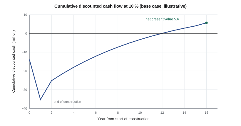
With immediate expensing, the line has an NPV of about 5.6 million Canadian dollars at 10 %, an internal rate of return of about 12.9 % and a payback of about 6.1 years after start-up. On the older Class 43 schedule, which still applies to machinery that comes into use after the full deduction steps down, the NPV would be about 4.1 million and the IRR about 11.9 %. The timing of start-up is worth about 1.5 million: a delay that pushed the line into service in 2030 would cut the first-year deduction to 75 %.
Measures of profitability
Each measure answers a different question. NPV answers how much value the project adds, in today's money, after paying for the capital at the company's required rate. It is the measure finance theory prefers, because it adds up across projects and is not fooled by scale. The internal rate of return, IRR, is the discount rate at which the NPV is exactly zero. It answers how much the project earns per dollar invested, which is easy to compare with the cost of capital, but it can mislead when comparing projects of very different sizes, and it can have more than one value when cash flows change sign more than once. Payback, the time to recover the initial investment from the cash flows, answers how long the money is at risk. It ignores what happens after payback, but Malik reports it because Kingfisher's board asks for it, and because a long payback on a small plant is a warning that the project depends on conditions holding for many years.
Worked problem
IRR and NPV
A project costs 10 million now and returns 1.5 million a year for 12 years after tax. Find its NPV at 10 % and estimate its IRR.
Show solution
- The annuity factor at 10 % for 12 years is \((1 - 1.1^{-12})/0.10 = 6.81\).
- NPV \(= -10 + 1.5 \times 6.81 = 0.22\) million.
- At 11 %, the factor is 6.49 and NPV \(= -0.26\) million.
- Interpolating, the IRR is about \(10 + 0.22/(0.22 + 0.26) = 10.5\) %.
Answer: NPV is about 0.2 million and the IRR about 10.5 %: a project that just clears its hurdle.
For the ester line, the three measures tell a consistent story. The project adds value, but not much. An IRR around 13 % against a 10 % cost of capital is a margin of only about three points. The payback of about six years is long for a plant whose margin depends on commodity price spreads. Malik's first comment to Theo is that a project like this lives or dies on its sensitivities, and the next part of the analysis is about them.
Sensitivity analysis
A sensitivity analysis changes one input at a time and records the effect on NPV. The inputs are chosen because they are uncertain and because they matter: the capital cost, over the AACE Class 3 range from lesson 7; the cash margin, which moves with the spread between the product and raw material prices; the discount rate; and the plant's life. The results are shown as a tornado chart, with the widest bar at the top.
| Change | NPV (million) |
|---|---|
| Base case | 5.64 |
| Capital +25 % | -0.79 |
| Capital -15 % | 9.50 |
| Margin -20 % | -0.99 |
| Margin +20 % | 12.27 |
| Discount rate 12 % | 1.52 |
| Discount rate 8 % | 10.69 |
| Life 10 years | -0.62 |
| Life 20 years | 9.53 |
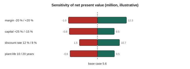
The margin is the widest bar, and a 20 % fall in the margin, which is only about 70 per tonne, turns the NPV negative. A 25 % capital overrun, at the top of the Class 3 range, does the same. So does a plant life of only ten years. Each of these is plausible on its own. The discount rate also matters, which is a reminder that the hurdle the company sets is part of the answer: at 12 % the project barely clears.
The tornado chart has a weakness: it moves one input at a time, while in reality several move together. Product and raw material prices are linked, as lesson 8 noted, so the margin swings less than either price; on the other hand, a capital overrun often comes with a late start-up, which delays the margin as well. For a fuller picture the team uses a Monte Carlo simulation.
Monte Carlo simulation
A Monte Carlo simulation draws each uncertain input from a probability distribution, runs the model, and repeats thousands of times. The result is a distribution of NPV rather than a single value. The code draws the capital from a triangular distribution between 85 % and 125 % of the estimate, matching the asymmetric Class 3 range, and the margin from a normal distribution with a standard deviation of 15 %, representing the spread between product and raw material prices. Five thousand trials are enough for the percentiles to settle.
The median NPV is about 4.7 million, lower than the base case because the capital range is skewed upward. The 10th percentile, the P10, is about minus 1.9 million and the 90th percentile, the P90, about 11.6 million. The chance of a negative NPV is about 18 %. In words: the project is more likely than not to create value, but about one time in five it will not earn its cost of capital.
A Monte Carlo result is only as good as its distributions, and Malik is careful to say so in the report. The 15 % spread in margin comes from Malik's review of a decade of price data, adjusted for the linkage between acid and ester. The capital range comes from the AACE class. Neither is precise, but both are better than pretending the base case is certain. The result also points to what could make the project safer: anything that narrows the margin distribution, such as a long-term acid contract, or that cuts the capital, or that raises the margin, such as lower steam use. Those are the options in lesson 12.
Common mistakes
MistakeMixing real cash flows with a nominal discount rate.
InsteadUse real with real or nominal with nominal, never a mix.
MistakeRanking projects of different size by IRR.
InsteadUse NPV to compare value; IRR favours small projects.
MistakeIgnoring the timing of tax deductions.
InsteadImmediate deductions are worth more in present value than slow ones.
MistakeReading a tornado chart as a full risk picture.
InsteadInputs move together; use Monte Carlo for combined uncertainty.
MistakePresenting the base case as the expected outcome.
InsteadWhen ranges are skewed, the median and mean differ from the base case.
Summary and key terms
- NPV discounts all cash flows at the cost of capital; positive NPV means the project adds value.
- The base case NPV is about 5.6 million with an IRR of about 12.9 % and a payback of about 6.1 years.
- Immediate deduction of capital is worth about 1.5 million against a slower schedule.
- Margin and capital cost are the largest sensitivities; a 20 % fall in margin makes NPV negative.
- Monte Carlo gives a median NPV of about 4.7 million and an 18 % chance of loss.
- Net present value
- The sum of all cash flows discounted at the cost of capital.
- Internal rate of return
- The discount rate that makes NPV zero.
- Payback
- The time for cash flows to recover the initial investment.
- Real terms
- Expressed in money of constant purchasing power, without inflation.
- Tornado chart
- A chart of the effect of each input alone on an output, widest bar first.
- Monte Carlo simulation
- Repeated model runs with inputs drawn from probability distributions.
- P10 and P90
- The values below which 10 % and 90 % of outcomes fall.
Practice problems
Work each problem on paper first, then reveal the answer to check.
What is the present value of 1 million received in 5 years at 10 %?
Show answer
About 0.62 million.
Why does immediate expensing increase NPV if the total deduction is unchanged?
Show answer
The tax saving comes earlier, so its present value is higher.
What does an IRR below the discount rate imply about NPV?
Show answer
NPV is negative.
Which single change in the tornado chart has the widest range?
Show answer
The margin.
Why is the Monte Carlo median below the base case?
Show answer
The capital range is skewed upward.
What two kinds of option could reduce the chance of loss?
Show answer
Narrowing the margin spread, for example with a contract, or improving the margin or capital.
Lesson quiz · 5 questions
Score 60% or more to complete this lesson.
Create a free account to save your progress, take quizzes and earn a certificate.