
CHE-446 · Lesson 7 of 12 · 21 min
Capital cost estimation
Lucia has the equipment list. Her job now is to turn it into a number: the fixed capital investment, the total cost of designing, buying, building and starting up the ester line, ready to make product. That number is the largest single input to the investment decision in lesson 9, and its accuracy is what separates one class of estimate from the next. In FEL-1 the team used a curve; in FEL-3 they build the estimate up from the equipment, item by item, and then apply factors for everything that goes around the equipment.
Every capital estimate, whatever its class, must state four things. What is included, and where the battery limits are. What date the prices refer to, because equipment prices change with the economy. What location, because labour costs and productivity differ widely from one place to another. And what accuracy it claims, which in practice means its AACE class. An estimate that omits any of these cannot be compared with another estimate, and Ingrid has seen investment decisions go wrong because two estimates from different years or sites were set side by side as if they were the same.
Estimating methods
There are four broad ways to estimate capital, in rising order of effort and accuracy. Capacity scaling uses the cost of a similar plant and scales it by size. The factored method prices the main equipment and multiplies by factors for installation, piping, instruments, electrical work, buildings and so on. The semi-detailed method adds material take-offs for the larger bulk items, such as piping and steel, priced separately. The detailed method prices everything from drawings and vendor quotes. FEL-1 used capacity scaling; FEL-3 for a small line like this one uses a factored estimate with vendor quotes for the major items and semi-detailed pricing for the largest bulk items.
Capacity scaling and cost indices
Plant and equipment costs grow less than linearly with size. A vessel twice as large needs less than twice the steel, because volume grows faster than surface area, and the cost of instruments, controls and engineering hardly changes with size at all. The usual expression is the six-tenths rule, in which cost scales as capacity to the power of about 0.6. The exponent varies by type of equipment and of plant, from about 0.4 for some compressors and tanks to near 1 for items that are added in parallel, such as large numbers of identical pumps or modules; 0.6 is a fair average for whole chemical plants.
The second ratio corrects for time. A cost index tracks how the price of a typical basket of plant equipment, materials and labour changes over time. The best known for chemical plants is the Chemical Engineering Plant Cost Index, CEPCI, published monthly by Chemical Engineering magazine. It stood near 500 in the early 2000s, rose sharply in 2021 and 2022 with the rise in steel and equipment prices, and has been around 800 in the mid-2020s. Lucia's FEL-1 estimate used a published reference cost for a 50,000 t/yr plant, indexed from a base of 500 to 800, and scaled to the ester line's capacity with an exponent of 0.6. The result was the 42.4 million Canadian dollars point estimate from lesson 1.
Location is the third correction. Published costs often refer to a US Gulf Coast plant, which is a common reference because the region builds many chemical plants. A location factor adjusts for differences in labour cost and productivity, climate, logistics and taxes. For Sarnia, Lucia uses the company's own record from the ethanol plant's last expansion rather than a published factor, because a site's own history is the best guide to what building there actually costs.
Worked problem
Scaling a reference plant
A reference ethyl acetate plant of 50,000 t/yr cost 46.9 million when the cost index was 500. Estimate the cost of a 19,300 t/yr plant today with the index at 800 and an exponent of 0.6.
Show solution
- Capacity ratio: \(19{,}300/50{,}000 = 0.386\); \(0.386^{0.6} = 0.565\).
- Index ratio: \(800/500 = 1.6\).
- Cost \(= 46.9 \times 1.6 \times 0.565 = 42.4\) million, before any location adjustment.
Answer: About 42.4 million, the FEL-1 point estimate from lesson 1; indexed to today, the reference plant itself would cost 75 million.
The factored estimate
A factored estimate starts with the purchased cost of each major item of equipment, delivered to site. Lucia prices the large items from vendor quotes received during FEL-3: the reactive column and its licensed packing, the ester column, the exchangers, the tanks. She prices smaller items from cost correlations in the company's database, adjusted to the current index. Each item is then multiplied by an installation factor that covers everything needed to put it into service: the foundation, the setting, the piping connected to it, the instruments, the electrical work, insulation and paint. Installation factors vary by type of equipment; a pump, with its piping and motor, has a higher factor than a large tank, which is mostly steel.
# Factored capital estimate for the ethyl acetate line (illustrative correlations and factors)
# Purchased cost Cp = a + b * S**n at a base cost index of 500; escalated to an index of 800
base_index, now_index = 500.0, 800.0
items = [  # name, a, b, n, size S (units in comment), count, installation factor
    ("pre-reactor vessel (m3 shell)",      12000, 21000, 0.60, 2.9,  1, 3.0),
    ("reactive distillation column (t shell)", 15000, 20000, 0.80, 18.0, 1, 3.6),
    ("ester column (t shell)",            15000, 20000, 0.80, 11.0, 1, 3.6),
    ("water stripper (t shell)",          15000, 20000, 0.80, 4.0,  1, 3.6),
    ("structured packing and internals (m3)", 0, 9500, 1.00, 48.0, 1, 1.8),
    ("decanter (m3)",                     10000, 30000, 0.55, 6.0,  1, 3.0),
    ("shell-and-tube exchangers (m2)",    28000, 1600, 0.85, 95.0,  6, 3.2),
    ("reboilers (m2)",                    30000, 1750, 0.85, 75.0,  3, 3.2),
    ("centrifugal pumps (L/s)",           8000, 2400, 0.80, 1.5,   8, 4.0),
    ("storage tanks (m3)",                5000, 1400, 0.70, 1000.0, 5, 2.4),
    ("nitrogen blanketing and vents (lot)", 0, 280000, 1.00, 1.0, 1, 2.0),
    ("control system, SIS and electrical (lot)", 0, 600000, 1.00, 1.0, 1, 2.0),
    ("pipe rack, structures and building (lot)", 0, 500000, 1.00, 1.0, 1, 2.0),
]
pce = isbl = 0.0
print("item                                       count   purchased each   installed (all)")
for n, a, b, ex, S, cnt, f in items:
    cp = (a + b * S ** ex) * now_index / base_index
    pce += cp * cnt; isbl += cp * cnt * f
    print(f"  {n:40s} {cnt:3d}   {cp/1e3:10.0f} k     {cp*cnt*f/1e6:7.2f} M")
osbl = 0.40 * isbl; dne = 0.25 * (isbl + osbl); cont = 0.15 * (isbl + osbl)
fci = isbl + osbl + dne + cont
print(f"\npurchased equipment cost   {pce/1e6:6.2f} million")
print(f"ISBL installed             {isbl/1e6:6.2f} million (overall factor {isbl/pce:.2f})")
print(f"OSBL at 40 %               {osbl/1e6:6.2f}")
print(f"design and engineering 25% {dne/1e6:6.2f}")
print(f"contingency 15 %           {cont/1e6:6.2f}")
print(f"fixed capital investment   {fci/1e6:6.2f} million")
print(f"Lang-factor check (4.74 x purchased) {4.74*pce/1e6:6.2f} million")
# Six-tenths rule check against a reference plant: 50,000 t/yr for 75 million at the same index
ref = 75e6 * (19317 / 50000) ** 0.6
print(f"six-tenths scaling of a 50 kt/yr reference plant: {ref/1e6:.1f} million")item count purchased each installed (all) pre-reactor vessel (m3 shell) 1 83 k 0.25 M reactive distillation column (t shell) 1 347 k 1.25 M ester column (t shell) 1 242 k 0.87 M water stripper (t shell) 1 121 k 0.44 M structured packing and internals (m3) 1 730 k 1.31 M decanter (m3) 1 145 k 0.43 M shell-and-tube exchangers (m2) 6 168 k 3.22 M reboilers (m2) 3 158 k 1.52 M centrifugal pumps (L/s) 8 18 k 0.58 M storage tanks (m3) 5 290 k 3.48 M nitrogen blanketing and vents (lot) 1 448 k 0.90 M control system, SIS and electrical (lot) 1 960 k 1.92 M pipe rack, structures and building (lot) 1 800 k 1.60 M purchased equipment cost 6.95 million ISBL installed 17.76 million (overall factor 2.56) OSBL at 40 % 7.10 design and engineering 25% 6.22 contingency 15 % 3.73 fixed capital investment 34.81 million Lang-factor check (4.74 x purchased) 32.94 million six-tenths scaling of a 50 kt/yr reference plant: 42.4 million
The code builds up the estimate. Thirteen lines of purchased equipment come to about 6.95 million Canadian dollars. Installed, with individual factors, they come to about 17.8 million inside battery limits, an overall installation factor of about 2.6. Outside battery limits, Lucia adds about 40 % of ISBL, or 7.1 million, for the new tie-ins to the site's steam, cooling water, nitrogen, flare and power systems, the rail spur extension, the dikes and roads, and the share of the control room upgrade. Design and engineering at 25 % adds 6.2 million. A contingency of 15 %, appropriate for an AACE Class 3 estimate of this definition, adds 3.7 million. The fixed capital investment comes to about 34.8 million Canadian dollars.
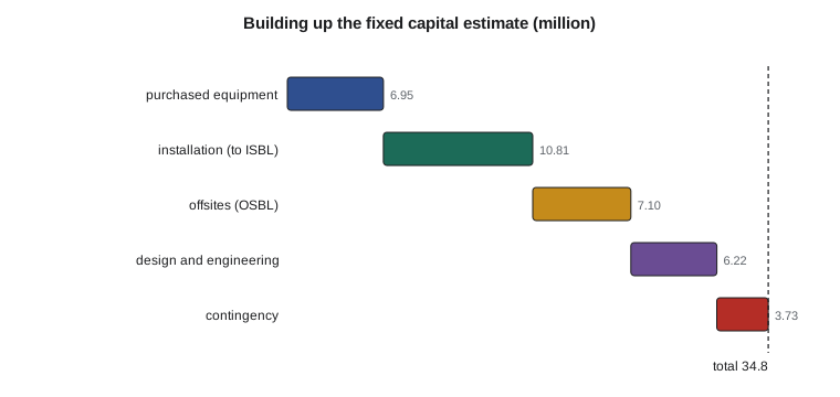
Two checks follow. The first is a Lang factor: the ratio of total plant cost to purchased equipment cost, which for fluid-processing plants is about 4 to 5. Using 4.74 gives about 32.9 million, close to the factored estimate, so the two methods agree. The second is the FEL-1 estimate. At 42.4 million, capacity scaling came in about 20 % higher than the factored estimate. That is well within the Class 5 range of minus 50 to plus 100 %, and the reason is clear: the reference plant was a standalone site, while the ester line shares utilities, a control room and a tank farm with the ethanol plant. Integration is the main source of value in the project, and it shows up first in the capital estimate.
| Component | Million | Share of FCI |
|---|---|---|
| Purchased equipment | 6.95 | 20 % |
| Installation (to ISBL) | 10.81 | 31 % |
| Outside battery limits | 7.10 | 20 % |
| Design and engineering | 6.22 | 18 % |
| Contingency | 3.73 | 11 % |
| Fixed capital investment | 34.81 | 100 % |
Contingency and accuracy
Contingency is often misunderstood. It is not a cushion for scope changes or a fund for things the project forgot; it is an allowance for costs that will certainly be incurred within the defined scope but cannot yet be priced exactly, such as quantities of pipe that will grow as the design develops, or prices that move before purchase. AACE's recommended practice treats contingency as the amount that brings the estimate to its expected value, and it is usually set by a risk analysis rather than a flat percentage. For Class 3, contingencies of about 10 to 20 % are common. Escalation, the rise in prices between the estimate date and the date of purchase, is a separate line. So is any allowance for scope that has not been defined, which a disciplined project keeps out of the estimate altogether and handles through change control.
The accuracy of the estimate is expressed as a range. For Class 3, AACE gives a typical range of about minus 10 to minus 20 % on the low side and plus 10 to plus 30 % on the high side, and lesson 1 used a range of about 36 to 53 million around a point estimate of 42.4 million to illustrate it. With the FEL-3 estimate at 34.8 million, the corresponding range is about 30 to 44 million. That range is what feeds the sensitivity analysis in lesson 9.
Working capital and other costs
The fixed capital investment is not the whole investment. Working capital is the money tied up in running the business: raw materials and product in the tanks, product shipped but not yet paid for, minus raw materials received but not yet paid for. It is recovered at the end of the project's life, but it must be found at start-up. For the ester line, with two to three weeks of storage and customers paying in about 30 days, Lucia estimates working capital at about 2.6 million Canadian dollars, close to the common rule of thumb of 10 to 15 % of FCI. Start-up costs, the first fill of catalyst and the initial spare parts are added to the project cost as well.
Tax treatment of capital depends on the jurisdiction. In Ontario the deduction is capital cost allowance. Federal legislation passed in March 2026 lets the full cost of eligible manufacturing and processing machinery acquired after 2024 be deducted in the year it becomes available for use, provided that is before 2030; the deduction then steps down to 75 % and 55 % and ends after 2033, when such machinery returns to Class 43 at 30 % a year on a declining balance with the half-year rule. A broader, permanent immediate expensing measure for most new capital property was proposed in September 2026. The ester line is scheduled to start up in 2029, so it falls inside the full deduction, but only if it is in use before 2030. Lesson 9 shows that the difference between these regimes is worth more than a million in net present value, which is large compared with the margins of a project like this one.
Common mistakes
MistakeComparing estimates from different years or sites without adjustment.
InsteadIndex both to the same date and correct for location.
MistakeTreating contingency as a fund for scope changes.
InsteadContingency covers defined scope that cannot yet be priced; new scope goes through change control.
MistakeUsing a single Lang factor for every plant.
InsteadFactors vary with plant type; item-by-item installation factors are better in FEL-3.
MistakeForgetting outside battery limits costs.
InsteadTie-ins, utilities and infrastructure can be 20 to 50 % of ISBL.
MistakeLeaving out working capital.
InsteadIt is part of the investment even though it is recovered at the end.
Summary and key terms
- Every estimate must state scope, date, location and class.
- Capacity scaling uses an exponent of about 0.6 and a cost index such as CEPCI.
- The FEL-3 factored estimate gives an FCI of about 34.8 million, with purchased equipment about a fifth of the total.
- Integration with the ethanol site explains why the estimate is below the FEL-1 standalone figure.
- Working capital of about 2.6 million is added to the fixed capital.
- Fixed capital investment
- The total cost of designing, building and commissioning the plant.
- ISBL
- Inside battery limits: the process plant itself.
- OSBL
- Outside battery limits: utilities, infrastructure and site connections.
- Lang factor
- The ratio of total plant cost to purchased equipment cost.
- Cost index
- A number that tracks the change in plant costs over time, such as CEPCI.
- Contingency
- An allowance for costs within defined scope that cannot yet be priced exactly.
- Working capital
- Money tied up in inventory and receivables, recovered at the end of the project.
Practice problems
Work each problem on paper first, then reveal the answer to check.
A plant cost 20 million at index 600. What does it cost at index 800, same size?
Show answer
About 26.7 million.
What does doubling capacity do to cost with an exponent of 0.6?
Show answer
Raises it by a factor of about 1.52.
What is the overall installation factor in the FEL-3 estimate?
Show answer
About 2.6.
Why is the FEL-3 estimate lower than FEL-1?
Show answer
The line shares utilities and infrastructure with the ethanol plant.
Is escalation part of contingency?
Show answer
No; it is a separate line.
Why must working capital be found at start-up even though it is recovered later?
Show answer
The tanks must be filled and customers pay after delivery.
Lesson quiz · 5 questions
Score 60% or more to complete this lesson.
Create a free account to save your progress, take quizzes and earn a certificate.