
CHE-220 · Lesson 9 of 12 · 24 min
Thermodynamic diagrams, tables and property software
For steam, ammonia and carbon dioxide, engineers rarely calculate properties from scratch. They read them from tables, diagrams or property software built on highly accurate fluid-specific equations of state. Kingfisher's boiler and turbine study runs on steam tables, the refrigeration plant on ammonia tables, and the liquefaction unit on carbon dioxide property software. Theo knows how to look numbers up, but Ingrid wants him to understand how those sources are built, how their reference states work, which diagrams suit which jobs, and how to check a number he does not trust. This lesson covers all four, and finishes by building a small carbon dioxide saturation table from the Peng-Robinson equation, the same way a property package does.
How steam tables are organized
Steam tables are the classic example. Modern tables come from the IAPWS formulations of the International Association for the Properties of Water and Steam: IAPWS-95 for scientific use and IAPWS-IF97, a faster industrial version, for engineering calculations. Both reproduce measured data within its experimental uncertainty over the ranges that matter for power and process plants. Printed tables and software built on them are organized the same way.
| Table | Entered by | Gives |
|---|---|---|
| Saturated water, temperature table | Temperature | Psat, V, U, H, S of saturated liquid and vapour, and differences such as hfg |
| Saturated water, pressure table | Pressure | Tsat and the same saturated properties |
| Superheated steam | Pressure and temperature | V, U, H, S of vapour above saturation |
| Compressed liquid | Pressure and temperature | V, U, H, S of liquid above saturation pressure |
| Saturated ice and vapour | Temperature | Properties for sublimation below the triple point |
Tables for other fluids follow the same pattern. For compressed liquids, when no table is available, a good approximation takes the saturated liquid values at the same temperature and corrects only the enthalpy for pressure, \(H \approx H^l_{sat}(T) + V^l(P - P^{sat})\), using the result from Lesson 8 with the small expansivity term neglected.
Interpolation
Tables list properties at intervals, so values in between come from interpolation. Linear interpolation is usually adequate in superheated steam tables when the intervals are 50 K or less, and in saturated tables. Double interpolation, first in temperature and then in pressure, is needed when both fall between entries. Property software removes the need for interpolation entirely, which is one reason it has largely replaced printed tables in design work, but interpolation remains essential for checking and for exam conditions.
Worked problem
Superheated steam for the turbine study
Kingfisher's turbine study considers steam at 4.0 MPa and 425 °C. Approximate table values at 4.0 MPa are \(H = 3213.6\ \text{kJ/kg}\), \(S = 6.7690\ \text{kJ/(kg·K)}\) at 400 °C and \(H = 3330.3\ \text{kJ/kg}\), \(S = 6.9363\ \text{kJ/(kg·K)}\) at 450 °C. Find \(H\) and \(S\) at 425 °C.
Show solution
- Fraction of the interval: \((425 - 400)/(450 - 400) = 0.5\).
- \(H = 3213.6 + 0.5 \times (3330.3 - 3213.6) = 3271.9\ \text{kJ/kg}\).
- \(S = 6.7690 + 0.5 \times (6.9363 - 6.7690) = 6.8527\ \text{kJ/(kg·K)}\).
Answer: Property software gives values within a fraction of a kJ/kg of these. Interpolation errors grow where properties curve strongly, close to the saturation curve and near the critical point, so use narrower intervals or software there.
Reference states
Tables report enthalpy, internal energy and entropy relative to an arbitrary reference state, because thermodynamics fixes only their changes. Steam tables set the internal energy and entropy of saturated liquid water at the triple point to zero. Refrigerant tables often use the convention of the International Institute of Refrigeration (IIR): \(H = 200\ \text{kJ/kg}\) and \(S = 1.000\ \text{kJ/(kg·K)}\) for saturated liquid at 0 °C. Other common conventions are the ASHRAE one, which sets \(H = 0\) and \(S = 0\) for saturated liquid at −40 °C, and the normal boiling point convention.
Changes in properties do not depend on the reference, so any table works for energy balances as long as all values come from the same source. Mixing sources is a classic error: enthalpies of ammonia from one table and from another can differ by hundreds of kJ/kg for the same state, simply because they use different references. If you must combine sources, shift one set by matching a common state, such as saturated liquid at 0 °C.
Thermodynamic diagrams
Diagrams show at a glance what tables show in numbers. Each suits a different job. A temperature-entropy diagram shows heat transfer as area under a reversible path, which makes it the natural diagram for power cycles. A pressure-enthalpy diagram makes the steps of a refrigeration cycle into straight lines: evaporation and condensation are horizontal lines at constant pressure, throttling is a vertical line at constant enthalpy, and the compressor work and refrigeration effect can be read directly as enthalpy differences. An enthalpy-entropy diagram, the Mollier chart, shows turbine expansions and nozzle flows, where both enthalpy change and departure from constant entropy matter.
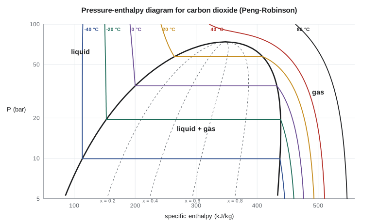
Diagrams have a practical advantage beyond quick reading: they make errors visible. A refrigeration cycle drawn on a P-h diagram with the compressor outlet inside the dome, or a turbine expansion drawn on an h-s diagram that loses entropy, is obviously wrong, while the same mistake in a spreadsheet can hide for months.
Property software
Modern design uses property libraries that implement reference equations of state, usually written in terms of the Helmholtz energy as a function of temperature and density. A Helmholtz equation for a fluid like carbon dioxide may have forty or more fitted terms, chosen so that every measured property, from densities to speeds of sound, is reproduced within its uncertainty. All other properties follow from the Helmholtz energy by differentiation, using the relations of Lesson 8, which guarantees that the whole set is thermodynamically consistent. Reference equations of this kind exist for water, carbon dioxide, ammonia, nitrogen, oxygen, methane and dozens of refrigerants and hydrocarbons.
Process simulators offer both reference equations and the simpler models of Lessons 3 to 5. The simpler models are faster and extend to mixtures, which is why they dominate in large flowsheets. A good habit is to check the simulator's choice for the key streams: if a cubic equation is used for liquid carbon dioxide in a tank-sizing calculation, its 2 to 10 percent density error goes straight into the tank volume.
Building a table from an equation of state
A saturation table needs vapour pressures. A cubic equation of state locates them as the pressure at which the liquid and vapour roots have the same fugacity coefficient, the condition for phase equilibrium developed fully in Thermodynamics II. Starting from a Lee-Kesler estimate, the pressure is corrected repeatedly by the ratio of the two fugacity coefficients until they match. Enthalpies and entropies then come from the ideal gas state plus the residual properties of Lesson 8, shifted to the chosen reference.
# A saturation table for carbon dioxide generated from the Peng-Robinson equation, and steam-table interpolation
import math
R = 8.314
def pr_state(T, P, Tc, Pc, w, phase="vap"):
    """Peng-Robinson: returns Z, residual enthalpy H^R (J/mol), residual entropy S^R (J/mol K), ln(fugacity coefficient)."""
    k = 0.37464 + 1.54226 * w - 0.26992 * w ** 2
    sa = 1 + k * (1 - math.sqrt(T / Tc))
    ac = 0.45724 * R ** 2 * Tc ** 2 / Pc
    a, b = ac * sa ** 2, 0.07780 * R * Tc / Pc
    dadT = -ac * k * sa / math.sqrt(T * Tc)
    A, B = a * P / (R * T) ** 2, b * P / (R * T)
    c2, c1, c0 = -(1 - B), A - 3 * B ** 2 - 2 * B, -(A * B - B ** 2 - B ** 3)
    p = c1 - c2 ** 2 / 3; q = 2 * c2 ** 3 / 27 - c2 * c1 / 3 + c0
    disc = (q / 2) ** 2 + (p / 3) ** 3
    if disc > 0:
        u, v = -q / 2 + math.sqrt(disc), -q / 2 - math.sqrt(disc)
        roots = [math.copysign(abs(u) ** (1 / 3), u) + math.copysign(abs(v) ** (1 / 3), v) - c2 / 3]
    else:
        r = math.sqrt(-(p / 3) ** 3); phi = math.acos(max(-1.0, min(1.0, -q / (2 * r)))); m = 2 * math.sqrt(-p / 3)
        roots = [m * math.cos((phi + 2 * math.pi * j) / 3) - c2 / 3 for j in range(3)]
    roots = sorted(z for z in roots if z > B)
    Z = roots[-1] if phase == "vap" else roots[0]
    L = math.log((Z + (1 + math.sqrt(2)) * B) / (Z + (1 - math.sqrt(2)) * B))
    HR = R * T * (Z - 1) + (T * dadT - a) / (2 * math.sqrt(2) * b) * L
    SR = R * math.log(Z - B) + dadT / (2 * math.sqrt(2) * b) * L
    lnphi = Z - 1 - math.log(Z - B) - A / (2 * math.sqrt(2) * B) * L
    return Z, HR, SR, lnphi

Tc, Pc, w, M = 304.2, 73.8e5, 0.224, 44.01            # carbon dioxide (approximate)
A_, B_, D_ = 5.457, 1.045e-3, -1.157e5

def psat(T):
    """Vapour pressure: start from Lee-Kesler, then equate liquid and vapour fugacities."""
    Tr = T / Tc
    f0 = 5.92714 - 6.09648 / Tr - 1.28862 * math.log(Tr) + 0.169347 * Tr ** 6
    f1 = 15.2518 - 15.6875 / Tr - 13.4721 * math.log(Tr) + 0.43577 * Tr ** 6
    P = Pc * math.exp(f0 + w * f1)
    for _ in range(200):
        lnphi_l = pr_state(T, P, Tc, Pc, w, "liq")[3]
        lnphi_v = pr_state(T, P, Tc, Pc, w, "vap")[3]
        P *= math.exp(lnphi_l - lnphi_v)
        if abs(lnphi_l - lnphi_v) < 1e-10: break
    return P

def h_s(T, P, phase):
    """Absolute-reference enthalpy and entropy per kg: ideal gas from 273.15 K and 1 bar plus residuals."""
    Z, HR, SR, _ = pr_state(T, P, Tc, Pc, w, phase)
    T0 = 273.15
    hig = R * (A_ * (T - T0) + B_ / 2 * (T ** 2 - T0 ** 2) - D_ * (1 / T - 1 / T0))
    sig = R * (A_ * math.log(T / T0) + B_ * (T - T0) - D_ / 2 * (1 / T ** 2 - 1 / T0 ** 2) - math.log(P / 1e5))
    return (hig + HR) / M, (sig + SR) / M, Z

# Shift to the refrigeration convention: saturated liquid at 0 C has h = 200 kJ/kg and s = 1.000 kJ/(kg K)
P0 = psat(273.15)
h0, s0, _ = h_s(273.15, P0, "liq")
print(" T (C)  Psat (bar)  rho_l (kg/m3)  rho_v   h_l     h_v   (kJ/kg)   s_l     s_v  (kJ/kg K)")
for t in (-50, -40, -30, -20, -10, 0, 10, 20, 25):
    T = t + 273.15
    P = psat(T)
    hl, sl, Zl = h_s(T, P, "liq"); hv, sv, Zv = h_s(T, P, "vap")
    rl, rv = P * M / 1000 / (Zl * R * T), P * M / 1000 / (Zv * R * T)
    print(f"{t:6.0f} {P/1e5:10.2f} {rl:12.0f} {rv:9.1f} {hl-h0+200:7.1f} {hv-h0+200:7.1f} {sl-s0+1:12.3f} {sv-s0+1:7.3f}")

# Linear interpolation in a steam table: superheated steam at 4 MPa (approximate table values)
table = {400: (3213.6, 6.7690), 450: (3330.3, 6.9363)}  # T (C): h (kJ/kg), s (kJ/kg K)
def interp(x, x1, y1, x2, y2): return y1 + (y2 - y1) * (x - x1) / (x2 - x1)
h425 = interp(425, 400, table[400][0], 450, table[450][0])
s425 = interp(425, 400, table[400][1], 450, table[450][1])
print(f"Steam at 4 MPa and 425 C by linear interpolation: h = {h425:.1f} kJ/kg, s = {s425:.4f} kJ/(kg K)") T (C) Psat (bar) rho_l (kg/m3) rho_v h_l h_v (kJ/kg) s_l s_v (kJ/kg K)
-50 6.77 1203 17.7 95.6 435.2 0.591 2.113
-40 9.94 1158 25.7 113.3 437.4 0.668 2.058
-30 14.13 1108 36.5 132.2 438.6 0.746 2.006
-20 19.52 1051 51.0 152.7 438.5 0.826 1.955
-10 26.31 987 70.7 175.1 436.7 0.910 1.905
0 34.73 912 97.6 200.0 432.3 1.000 1.851
10 44.99 822 136.3 228.7 424.2 1.099 1.789
20 57.36 705 197.2 264.4 409.0 1.217 1.710
25 64.42 627 246.4 287.7 395.9 1.292 1.655
Steam at 4 MPa and 425 C by linear interpolation: h = 3271.9 kJ/kg, s = 6.8527 kJ/(kg K)The generated table agrees well with reference-quality tables for carbon dioxide at low temperatures: at −20 °C the vapour pressure is within about 1 percent and the latent heat of about 286 kJ/kg is within a few percent. Near the critical point the cubic equation's limits show. At 20 °C it gives a liquid density of about 705 kg/m³ where reference tables give about 770 kg/m³. For the liquefaction plant, which condenses at −20 °C, Peng-Robinson is good enough for screening, but tank and truck capacities must come from reference data.
Worked problem
Reading a two-phase state from the table
Liquid carbon dioxide at 20 bar and −20 °C flows through a valve into a tank held at 14.1 bar, the vapour pressure at −30 °C. The valve is adiabatic, so enthalpy is constant. Using the generated table, with \(H^l = 152.7\ \text{kJ/kg}\) at −20 °C and \(H^l = 132.2\), \(H^v = 438.6\ \text{kJ/kg}\) at −30 °C, find the fraction that flashes to vapour.
Show solution
- The inlet liquid is nearly saturated, so take its enthalpy as the saturated liquid value at −20 °C: 152.7 kJ/kg.
- At the outlet, \(H = H^l + x(H^v - H^l)\): \(152.7 = 132.2 + x(438.6 - 132.2)\).
- \(x = 20.5/306.4 = 0.067\), so about 6.7 percent of the liquid flashes.
Answer: Letting liquid down by about 6 bar flashes almost 7 percent of it, and the vapour must be vented or recompressed. Lakeshore Gas keeps the transfer pressure drops small for this reason, and returns the flash vapour from tanker loading to the compressor suction rather than venting it.
Common mistakes
MistakeCombining enthalpies from tables with different reference states.
InsteadUse one source, or shift one set to match the other at a common state.
MistakeInterpolating linearly across wide intervals near saturation.
InsteadUse finer tables or software where properties curve strongly.
MistakeUsing saturated liquid enthalpy for a compressed liquid at very high pressure without correction.
InsteadAdd V^l(P − Psat) to the saturated enthalpy, or use a compressed liquid table.
MistakeTrusting cubic-equation densities near the critical point for sizing.
InsteadUse reference equations or measured data there.
MistakeDrawing a refrigeration cycle on a T-s diagram and reading work as enthalpy differences directly.
InsteadP-h diagrams show enthalpy differences directly; T-s diagrams show heat as areas.
Summary and key terms
- Steam tables come from IAPWS formulations and are organized as saturated, superheated and compressed liquid tables.
- Linear interpolation is adequate at modest intervals away from saturation and the critical point.
- Reference states are arbitrary; only property changes matter, so never mix sources without shifting.
- T-s diagrams suit power cycles, P-h diagrams refrigeration cycles, and h-s (Mollier) diagrams turbines and nozzles.
- Property software uses reference Helmholtz-energy equations, consistent through the property relations.
- A cubic equation can generate a saturation table by equating liquid and vapour fugacity coefficients.
- Steam tables
- Tabulated properties of water and steam from the IAPWS formulations.
- Reference state
- An arbitrary state at which H, U or S is assigned a fixed value for tabulation.
- Interpolation
- Estimating a value between tabulated entries, usually linearly.
- Mollier diagram
- An enthalpy-entropy diagram, used for turbines and nozzles.
- Pressure-enthalpy diagram
- A diagram on which refrigeration cycle steps appear as straight lines.
- Helmholtz energy equation
- A reference equation of state giving A(T, ρ), from which all other properties follow.
Practice problems
Work each problem on paper first, then reveal the answer to check.
Steam at 4 MPa: H = 3213.6 kJ/kg at 400 °C and 3330.3 kJ/kg at 450 °C. Find H at 410 °C.
Show answer
3213.6 + 0.2 × 116.7 = 3237.0 kJ/kg.
Two ammonia tables give saturated liquid enthalpy at 0 °C as 200.0 and 180.4 kJ/kg. How do you combine them?
Show answer
Subtract 19.6 kJ/kg from every enthalpy in the first table, or add it to the second, before mixing values.
From the program, what is the latent heat of carbon dioxide at −20 °C?
Show answer
About 438.5 − 152.7 = 286 kJ/kg.
Which diagram shows a throttling valve as a vertical line?
Show answer
The pressure-enthalpy diagram.
Estimate the enthalpy of compressed water at 10 MPa and 100 °C, given saturated H = 419.0 kJ/kg, V = 0.001044 m³/kg and Psat = 0.101 MPa.
Show answer
419.0 + 0.001044 × (10 000 − 101) = 419.0 + 10.3 = 429.3 kJ/kg.
Why do reference equations of state give thermodynamically consistent properties?
Show answer
All properties are derived from one Helmholtz energy function by exact property relations.
Lesson quiz · 5 questions
Score 60% or more to complete this lesson.
Create a free account to save your progress, take quizzes and earn a certificate.