Generalized correlations for gases and liquids

Equations of state need parameters, and sometimes the parameters are all you have. When Ingrid's team sized the new ammonia refrigeration plant, they needed vapour densities at the compressor suction and discharge and liquid densities in the receiver. They also needed the density of hot ethanol-rich liquid in the distillation reflux drums, where a level instrument calibrated for the wrong density reads wrongly. Measured data exist for all of these fluids, but engineers also need methods that work from a handful of constants, both for quick checks and for fluids without good data. This lesson covers the generalized, or corresponding-states, correlations that do that job for gases and liquids.

The principle of corresponding states

Van der Waals noticed that if you express pressure, volume and temperature as fractions of their critical values, the PVT behaviour of many fluids looks nearly the same. That observation is the two-parameter theorem of corresponding states: all fluids, compared at the same reduced temperature and reduced pressure, have about the same compressibility factor. It works very well for simple, spherical molecules such as argon, krypton and methane, and reasonably for many others, but it cannot capture the differences caused by molecular shape and polarity.

Pitzer's three-parameter version adds the acentric factor from Lesson 2. The compressibility factor becomes a simple-fluid value plus a correction proportional to \(\omega\). Both functions, \(Z^0\) and \(Z^1\), are universal: the same tables or charts serve every fluid. This is the same structure as the Pitzer virial correlation in Lesson 3 and the Lee-Kesler vapour pressure correlation in Lesson 2, and it explains why so many correlations need only \(T_c\), \(P_c\) and \(\omega\).

The Lee-Kesler correlation

The most widely used tables of \(Z^0\) and \(Z^1\) come from the Lee-Kesler correlation of 1975, which fitted an elaborate equation of state with twelve constants to data for a simple fluid and for a heavy reference fluid. The resulting tables cover reduced temperatures from about 0.3 to 4 and reduced pressures up to 10, in both gas and liquid regions, and similar tables give generalized enthalpy and entropy departures. For non-polar and slightly polar gases, Lee-Kesler compressibility factors are usually within 2 to 3 percent of measured values, rather better than a cubic equation near the critical point.

Using the tables means double interpolation in reduced temperature and pressure, which is tedious by hand and easy in software. Many process simulators offer Lee-Kesler, or its extension to mixtures by Plöcker and coworkers, as an option for light hydrocarbon systems. For hand calculations, a practical route is to use the Pitzer virial correlation where \(Z\) stays above about 0.85, and a cubic equation of state or the tables elsewhere.

Reading a generalized chart

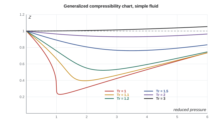
The chart shows the features that every engineer should recognize. All curves start at \(Z = 1\) at zero pressure, the ideal gas limit. Near the critical temperature, \(Z\) drops steeply as pressure rises toward the critical pressure, reaching values of about 0.25 to 0.3, because near-critical fluids are highly compressible: a small pressure change produces a large density change. At higher reduced temperatures, the dip is shallower, and above a reduced temperature of about 2.5 to 3, \(Z\) stays close to 1 and even rises above it at high pressures, as repulsion between molecules takes over. At very high reduced pressures, all curves rise with pressure for the same reason.

Two rules of thumb follow. A gas is close to ideal when its reduced pressure is small, say below 0.05, or when its reduced temperature is high, say above 2. And near the critical point, no simple correlation is reliable, so measured data or a reference equation should be used when accuracy matters. Nitrogen at room temperature has a reduced temperature of about 2.4, which is why it behaves almost ideally even at tens of bar. Carbon dioxide at room temperature has a reduced temperature of only about 0.97, which is why the liquefaction plant needs real-gas methods.

Liquid densities: the Rackett equation

Cubic equations of state give poor liquid densities, as Lesson 4 showed. For saturated liquids, the Rackett equation is a simple and widely used alternative. It needs the critical volume and critical compressibility factor, and it captures the way liquid density falls as temperature rises toward the critical point, where it meets the vapour density.

With the true critical compressibility factor, the Rackett equation is accurate to a few percent for non-polar liquids, but it does worse for polar and hydrogen-bonded liquids such as water and alcohols. A simple fix, due to Spencer and Danner, replaces \(Z_c\) with an adjustable parameter \(Z_{RA}\) fitted to one or more measured liquid densities. Fitted from a single density near room temperature, the modified equation then predicts densities over a wide temperature range to about 1 or 2 percent.

# Generalized correlations: Rackett liquid densities and Pitzer virial estimates for gases
import math
R = 8.314
# Tc (K), Pc (bar), omega, Vc (cm3/mol), Zc, molar mass (g/mol); approximate literature values
data = {"carbon dioxide": (304.2, 73.8, 0.224, 94.0, 0.274, 44.01),
        "ammonia":        (405.7, 112.8, 0.253, 72.5, 0.242, 17.03),
        "ethanol":        (513.9, 61.5, 0.645, 167.0, 0.240, 46.07),
        "water":          (647.1, 220.6, 0.345, 55.9, 0.229, 18.02)}

def rackett(T, Tc, Vc, Zc):
    """Saturated liquid molar volume (cm3/mol)."""
    return Vc * Zc ** ((1 - T / Tc) ** (2 / 7))

checks = [("carbon dioxide", -20, 1032), ("ammonia", -10, 652), ("ethanol", 20, 789),
          ("ethanol", 78, 736), ("water", 25, 997), ("water", 150, 917)]
print("Rackett saturated liquid densities (measured values approximate)")
for name, t, meas in checks:
    Tc, Pc, w, Vc, Zc, M = data[name]
    V = rackett(t + 273.15, Tc, Vc, Zc)
    rho = M / V * 1000
    print(f"  {name:15s} {t:5.0f} C  {rho:7.1f} kg/m3  measured {meas:5.0f}  error {100*(rho-meas)/meas:+5.1f} %")

# One-point fit: back out an effective Rackett parameter Z_RA from one measured density, then extrapolate
Tc, Pc, w, Vc, Zc, M = data["ethanol"]
V20 = M / 789 * 1000                                   # cm3/mol at 20 C
ZRA = (V20 / Vc) ** (1 / (1 - 293.15 / Tc) ** (2 / 7))
for t, meas in ((50, 763), (78, 736)):
    rho = M / rackett(t + 273.15, Tc, Vc, ZRA) * 1000
    print(f"  ethanol with fitted Z_RA = {ZRA:.4f}: {t} C {rho:6.1f} kg/m3, measured about {meas}, error {100*(rho-meas)/meas:+.1f} %")

def z_pitzer(T, P, Tc, Pc, w):
    Tr, Pr = T / Tc, P / Pc
    B0 = 0.083 - 0.422 / Tr ** 1.6
    B1 = 0.139 - 0.172 / Tr ** 4.2
    return 1 + (B0 + w * B1) * Pr / Tr, Tr, Pr

print("Ammonia vapour in the refrigeration plant (Pitzer virial)")
for label, t, p in (("evaporator outlet", -10, 2.9), ("compressor discharge", 110, 13.5), ("condenser inlet", 35, 13.5)):
    Tc, Pc, w, Vc, Zc, M = data["ammonia"]
    z, Tr, Pr = z_pitzer(t + 273.15, p, Tc, Pc, w)
    rho = p * 1e5 * M / 1000 / (z * R * (t + 273.15))
    ok = "inside" if z > 0.85 else "outside"
    print(f"  {label:21s} Tr = {Tr:.3f} Pr = {Pr:.4f}  Z = {z:.4f}  density {rho:6.2f} kg/m3 ({ok} the virial range)")

Rackett saturated liquid densities (measured values approximate)
  carbon dioxide    -20 C   1018.7 kg/m3  measured  1032  error  -1.3 %
  ammonia           -10 C    672.8 kg/m3  measured   652  error  +3.2 %
  ethanol            20 C    846.3 kg/m3  measured   789  error  +7.3 %
  ethanol            78 C    770.8 kg/m3  measured   736  error  +4.7 %
  water              25 C   1109.1 kg/m3  measured   997  error +11.2 %
  water             150 C    957.4 kg/m3  measured   917  error  +4.4 %
  ethanol with fitted Z_RA = 0.2624: 50 C  755.8 kg/m3, measured about 763, error -0.9 %
  ethanol with fitted Z_RA = 0.2624: 78 C  722.8 kg/m3, measured about 736, error -1.8 %
Ammonia vapour in the refrigeration plant (Pitzer virial)
  evaporator outlet     Tr = 0.649 Pr = 0.0257  Z = 0.9606  density   2.35 kg/m3 (inside the virial range)
  compressor discharge  Tr = 0.944 Pr = 0.1197  Z = 0.9494  density   7.60 kg/m3 (inside the virial range)
  condenser inlet       Tr = 0.760 Pr = 0.1197  Z = 0.8936  density  10.04 kg/m3 (inside the virial range)

The program shows the pattern clearly. With the true \(Z_c\), Rackett is within about 1 percent for carbon dioxide but 7 percent off for ethanol and 11 percent off for water at room temperature. With one fitted parameter, ethanol comes within 1 to 2 percent over the whole range. For ammonia vapour, the Pitzer correlation stays inside its range at all three points in the refrigeration plant.

Compressed liquids

The Rackett equation gives saturated liquid volumes. For liquids at pressures above saturation, the correction is usually small, because liquids are nearly incompressible, and it can be estimated from the isothermal compressibility or from correlations such as the Tait equation. For liquid carbon dioxide at −20 °C, raising the pressure from its vapour pressure of 19.6 bar to 30 bar increases the density by roughly 1 percent, while for liquid water near room temperature the same pressure rise changes the density by less than 0.1 percent. Liquids close to their critical points are much more compressible, and there the correction can be significant.

When to use which method

Generalized correlations are tools for estimation, checking and screening. They are excellent when you need a quick, defensible number for a gas at moderate pressure or a liquid near saturation, and when no better data are available. For final designs, regulatory reporting and custody transfer, engineers turn to measured data or reference-quality equations of state where those exist: the IAPWS formulation for water, and the reference equations for carbon dioxide, ammonia, nitrogen and many refrigerants that sit behind modern property software. Knowing a corresponding-states estimate also protects you from errors in that software: if a simulator reports a carbon dioxide density at 20 bar and 35 °C that is 20 percent away from the virial estimate, something in the setup is wrong.