
CHE-220 · Lesson 4 of 12 · 24 min
Cubic equations of state
The later stages of the Lakeshore Gas compressor run between 10 and 20 bar, the condenser holds liquid carbon dioxide near its saturation curve, and the company is also studying an option to deliver carbon dioxide by pipeline at 60 to 80 bar. The truncated virial equation cannot cover that range, and it says nothing at all about liquids. Ingrid asks Theo to set up a single equation that gives reasonable gas and liquid densities everywhere on the route. The answer, used inside nearly every process simulator, is a cubic equation of state.
From van der Waals to modern cubics
In 1873 Johannes van der Waals proposed the first equation of state able to describe both gas and liquid. He corrected the ideal gas law for the two molecular effects described in Lesson 3. Molecules take up space, so the volume available for motion is \(V - b\) rather than \(V\), where \(b\) is a co-volume related to molecular size. Molecules attract each other, which lowers the pressure they exert on the walls by an amount proportional to the square of the density, \(a/V^2\).
Written in terms of volume, the equation is a cubic polynomial. At high temperature it has one real root, a gas. Below the critical temperature, over a range of pressures, it has three real roots: the smallest is a liquid-like volume, the largest a vapour-like volume, and the middle one has no physical meaning. The van der Waals equation is too crude for engineering accuracy, but its structure, a repulsive term plus an attractive term, survives in every cubic equation used today.
The Redlich-Kwong equation of 1949 improved the attractive term and gave much better gas-phase results. Soave in 1972 made the attractive parameter depend on temperature through a function that brings in the acentric factor, which greatly improved vapour pressures. Peng and Robinson in 1976 changed the attractive term again to improve liquid densities. The Soave-Redlich-Kwong (SRK) and Peng-Robinson (PR) equations remain the workhorses of process design for hydrocarbons, gases and many other non-polar and mildly polar fluids.
The generic cubic
All four equations fit one generic form with two pure numbers, \(\sigma\) and \(\varepsilon\), that distinguish them. The parameters \(a\) and \(b\) come from the critical constants, and the temperature dependence of \(a\) enters through a function \(\alpha(T_r, \omega)\) that equals 1 at the critical temperature.
| Equation | σ | ε | Ω | Ψ | α(Tr) |
|---|---|---|---|---|---|
| van der Waals (1873) | 0 | 0 | 1/8 | 27/64 | 1 |
| Redlich-Kwong (1949) | 1 | 0 | 0.08664 | 0.42748 | Tr^(−1/2) |
| Soave-Redlich-Kwong (1972) | 1 | 0 | 0.08664 | 0.42748 | [1 + m(1 − Tr^(1/2))]², m = 0.480 + 1.574ω − 0.176ω² |
| Peng-Robinson (1976) | 1 + √2 | 1 − √2 | 0.07780 | 0.45724 | [1 + κ(1 − Tr^(1/2))]², κ = 0.37464 + 1.54226ω − 0.26992ω² |
The numbers \(\Omega\) and \(\Psi\) are not arbitrary. They come from forcing each equation to satisfy the two critical-point conditions from Lesson 2, zero slope and zero curvature of the critical isotherm at the critical point. That is why only \(T_c\), \(P_c\) and, for the modern equations, \(\omega\) are needed. It also means each equation predicts a single critical compressibility factor for every fluid, 0.375 for van der Waals, 0.333 for Redlich-Kwong and SRK, and 0.307 for Peng-Robinson, while real fluids range from about 0.23 to 0.29. Liquid densities near the critical point therefore carry errors that no choice of \(\alpha\) can remove.
Solving for Z
In practice, cubic equations are solved for the compressibility factor rather than the volume. Define two dimensionless groups, \(\beta = bP/(RT)\) and \(q = a/(bRT)\). Then the generic equation becomes a cubic polynomial in \(Z\) whose coefficients depend only on \(\beta\), \(q\), \(\sigma\) and \(\varepsilon\). For Peng-Robinson, it is often written with \(A = q\beta = aP/(RT)^2\) and \(B = \beta\).
When the cubic has three real roots, the largest belongs to the vapour and the smallest to the liquid. Which one is physically stable depends on whether the pressure is above or below the vapour pressure: below it the vapour root is stable, above it the liquid root. At the vapour pressure itself, both phases are in equilibrium. Lesson 9 and Thermodynamics II show how the equation locates that pressure by equating the fugacities of the two phases. Roots smaller than \(\beta\) are rejected because they would make \(V - b\) negative.
Worked problem
Peng-Robinson for compressed carbon dioxide gas
Find \(Z\) and the density of carbon dioxide at 20 bar and 35 °C with the Peng-Robinson equation. Use \(T_c = 304.2\ \text{K}\), \(P_c = 73.8\ \text{bar}\) and \(\omega = 0.224\).
Show solution
- \(\kappa = 0.37464 + 1.54226(0.224) - 0.26992(0.224)^2 = 0.7066\); \(T_r = 308.15/304.2 = 1.0130\); \(\alpha = [1 + 0.7066(1 - \sqrt{1.0130})]^2 = 0.9909\).
- \(a = 0.45724 \times 0.9909 \times 8.314^2 \times 304.2^2/(73.8\times10^5) = 0.3927\ \text{Pa·m}^6\text{/mol}^2\); \(b = 0.07780 \times 8.314 \times 304.2/(73.8\times10^5) = 2.666\times10^{-5}\ \text{m}^3\text{/mol}\).
- \(A = aP/(RT)^2 = 0.1197\); \(B = bP/(RT) = 0.02081\).
- Solve \(Z^3 - (1 - B)Z^2 + (A - 3B^2 - 2B)Z - (AB - B^2 - B^3) = 0\). Starting from \(Z = 1\), Newton's method converges to \(Z = 0.896\).
- Density \(= PM/(ZRT) = 20\times10^5 \times 0.04401/(0.896 \times 8.314 \times 308.15) = 38.3\ \text{kg/m}^3\).
Answer: The answer is within about 1 percent of the measured value of roughly 38 kg/m³. At this state, a moderate distance from the critical point, all the modern cubics agree closely, and so does the virial equation from Lesson 3.
Worked problem
The liquid in the condenser
Liquid carbon dioxide leaves the condenser at −20 °C and 20 bar, just above its vapour pressure. Its measured density is about 1032 kg/m³. Compare the liquid densities from the four cubic equations.
Show solution
- At these conditions each cubic has three real roots or one small root; take the smallest root above \(\beta\) as the liquid.
- The program gives \(Z_l\) = 0.068 (van der Waals), 0.047 (Redlich-Kwong), 0.045 (SRK) and 0.040 (Peng-Robinson).
- Densities: 617, 883, 927 and 1052 kg/m³, errors of about −40, −14, −10 and +2 percent.
Answer: Van der Waals is useless for liquids. SRK, excellent for vapour pressures, underpredicts liquid density by about 10 percent. Peng-Robinson does much better here, which is the main reason it was developed. For liquid volumes that must be accurate to a percent, such as custody transfer of liquid carbon dioxide into trucks, engineers apply a volume translation to the cubic or use a dedicated liquid-density correlation such as the Rackett equation from Lesson 5.
# Generic cubic equation of state: van der Waals, Redlich-Kwong, Soave-Redlich-Kwong and Peng-Robinson
import math
R = 8.314
Tc, Pc, w, M = 304.2, 73.8e5, 0.224, 44.01      # carbon dioxide (approximate)

def alpha(eos, Tr):
    if eos == "vdW": return 1.0
    if eos == "RK": return Tr ** -0.5
    if eos == "SRK":
        m = 0.480 + 1.574 * w - 0.176 * w ** 2
        return (1 + m * (1 - Tr ** 0.5)) ** 2
    k = 0.37464 + 1.54226 * w - 0.26992 * w ** 2  # Peng-Robinson
    return (1 + k * (1 - Tr ** 0.5)) ** 2

PARAMS = {"vdW": (0, 0, 1 / 8, 27 / 64), "RK": (1, 0, 0.08664, 0.42748),
          "SRK": (1, 0, 0.08664, 0.42748), "PR": (1 + 2 ** 0.5, 1 - 2 ** 0.5, 0.07780, 0.45724)}

def z_roots(eos, T, P):
    sig, eps, Om, Psi = PARAMS[eos]
    a = Psi * alpha(eos, T / Tc) * R ** 2 * Tc ** 2 / Pc
    b = Om * R * Tc / Pc
    beta, q = b * P / (R * T), a / (b * R * T)
    c2 = (eps + sig) * beta - 1 - beta
    c1 = eps * sig * beta ** 2 - (eps + sig) * beta * (1 + beta) + q * beta
    c0 = -(eps * sig * beta ** 2 * (1 + beta) + q * beta ** 2)
    p = c1 - c2 ** 2 / 3; qq = 2 * c2 ** 3 / 27 - c2 * c1 / 3 + c0
    disc = (qq / 2) ** 2 + (p / 3) ** 3
    if disc > 0:                                  # one real root
        u = -qq / 2 + math.sqrt(disc); v = -qq / 2 - math.sqrt(disc)
        roots = [math.copysign(abs(u) ** (1 / 3), u) + math.copysign(abs(v) ** (1 / 3), v) - c2 / 3]
    else:                                         # three real roots
        r = math.sqrt(-(p / 3) ** 3); phi = math.acos(-qq / (2 * r)); m = 2 * math.sqrt(-p / 3)
        roots = [m * math.cos((phi + 2 * math.pi * j) / 3) - c2 / 3 for j in range(3)]
    return sorted(z for z in roots if z > beta)

cases = [("gas, 20 bar, 35 C", 308.15, 20e5, "vap", 37.9),
         ("liquid, 20 bar, -20 C", 253.15, 20e5, "liq", 1032.0),
         ("dense gas, 60 bar, 40 C", 313.15, 60e5, "vap", 150.0)]
for label, T, P, ph, rho_ref in cases:
    print(f"{label}  (approximate reference density {rho_ref:.0f} kg/m3)")
    for eos in PARAMS:
        zs = z_roots(eos, T, P)
        z = zs[-1] if ph == "vap" else zs[0]
        rho = P * M / 1000 / (z * R * T)
        print(f"   {eos:4s} Z = {z:.4f}  density = {rho:7.1f} kg/m3  error {100 * (rho - rho_ref) / rho_ref:+6.1f} %")

print("Roots at saturation, -20 C and 19.6 bar (Peng-Robinson):",
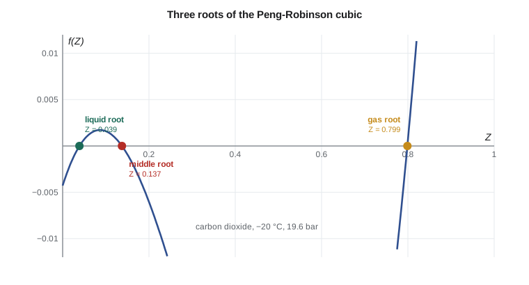
", ".join(f"{z:.4f}" for z in z_roots("PR", 253.15, 19.6e5)))gas, 20 bar, 35 C (approximate reference density 38 kg/m3) vdW Z = 0.9163 density = 37.5 kg/m3 error -1.1 % RK Z = 0.9055 density = 37.9 kg/m3 error +0.1 % SRK Z = 0.9060 density = 37.9 kg/m3 error +0.1 % PR Z = 0.8961 density = 38.3 kg/m3 error +1.2 % liquid, 20 bar, -20 C (approximate reference density 1032 kg/m3) vdW Z = 0.0678 density = 617.0 kg/m3 error -40.2 % RK Z = 0.0474 density = 883.1 kg/m3 error -14.4 % SRK Z = 0.0451 density = 926.6 kg/m3 error -10.2 % PR Z = 0.0398 density = 1051.8 kg/m3 error +1.9 % dense gas, 60 bar, 40 C (approximate reference density 150 kg/m3) vdW Z = 0.7029 density = 144.3 kg/m3 error -3.8 % RK Z = 0.6800 density = 149.2 kg/m3 error -0.6 % SRK Z = 0.6868 density = 147.7 kg/m3 error -1.5 % PR Z = 0.6609 density = 153.5 kg/m3 error +2.3 % Roots at saturation, -20 C and 19.6 bar (Peng-Robinson): 0.0390, 0.1374, 0.7988
The program confirms the pattern. For moderately compressed gas, every equation is within about 1 percent. In the dense gas at 60 bar and 40 °C, just above the critical temperature, the errors grow to a few percent for all of them, because near-critical fluids are the hardest region for any simple equation. For the liquid, only Peng-Robinson is close. The last line shows the three Peng-Robinson roots at the vapour pressure at −20 °C: about 0.039 for the liquid, 0.137 for the meaningless middle root and 0.799 for the vapour.
Practical tips for solving cubics
Cubic polynomials can be solved exactly with the trigonometric or Cardano formulas, which is what the program does, but iterative methods are common in spreadsheets and simulators. Two starting guesses cover most cases. For a vapour root, start Newton's method from \(Z = 1\), the ideal gas value, and it will usually descend to the largest root. For a liquid root, start from \(Z = \beta\), just above the smallest allowed value, and it will climb to the smallest root. If the two iterations converge to the same number, the cubic has only one real root at that state, and the fluid is either a gas, a liquid far from saturation or a supercritical fluid.
Check the result against physical sense before using it. A vapour \(Z\) above 1 at moderate pressure, or a liquid \(Z\) above about 0.3, signals that the wrong root or the wrong phase was picked. Also check units: \(a\) and \(b\) must use the same gas constant and pressure units as the rest of the calculation, and pressures must be absolute. A common spreadsheet error is to compute \(b\) with pressure in bar and then use it with pressure in pascals, which shifts \(\beta\) by a factor of 100 000.
Mixtures
Cubic equations extend to mixtures through mixing rules for \(a\) and \(b\). The classical van der Waals one-fluid rules take the mixture \(b\) as a mole-fraction average and the mixture \(a\) as a quadratic sum over pairs, with the cross term from a geometric mean corrected by a binary interaction parameter \(k_{ij}\) fitted to phase equilibrium data. For carbon dioxide with methane, \(k_{ij}\) is around 0.1, a small number that makes a large difference to predicted phase behaviour.
Lakeshore Gas's feed is not quite pure: it carries small amounts of oxygen, nitrogen, ethanol and water from the fermenters. Those impurities matter, because inert gases that cannot condense accumulate in the condenser and must be vented, and water must be removed before the gas is chilled or it will freeze or form hydrates. The company's process simulator uses Peng-Robinson with fitted interaction parameters for the gas phase, and a separate model for water and ethanol, which strongly polar molecules make difficult for any cubic equation.
Choosing an equation of state
No equation of state is best everywhere. A practical guide for second-year work, and for many design decisions, runs as follows. For gases at low pressure, use the ideal gas law. For gases at moderate pressure with \(Z\) above about 0.85, use the truncated virial equation, ideally with measured second virial coefficients. For gases and liquids over wide ranges, especially hydrocarbons and light gases, use Peng-Robinson or SRK. For accurate liquid densities, use Rackett or a volume-translated cubic. For water and steam, use the steam tables, which come from a highly accurate fluid-specific equation (Lesson 9). For refrigerants, carbon dioxide and other fluids with reference-quality equations, use those equations when accuracy matters, as in custody transfer or in the final design of the liquefaction plant.
Common mistakes
MistakeTaking the middle root of a cubic as a physical volume.
InsteadUse the largest root for vapour and the smallest for liquid; the middle root has no physical meaning.
MistakeUsing van der Waals for engineering calculations.
InsteadIt shows the right qualitative behaviour but is far too inaccurate, especially for liquids.
MistakeTrusting cubic liquid densities to a percent.
InsteadSRK typically underpredicts liquid densities by about 10 percent; use volume translation or Rackett.
MistakeForgetting the temperature dependence of a.
InsteadIn SRK and PR, a depends on temperature through α(Tr, ω); compute it at the actual temperature.
MistakeApplying cubic equations to water and alcohols without question.
InsteadStrongly polar, hydrogen-bonding fluids need steam tables or specialized models.
Summary and key terms
- Cubic equations combine a repulsive term RT/(V − b) with an attractive term in a(T).
- Van der Waals, Redlich-Kwong, SRK and Peng-Robinson share one generic form with different σ, ε, Ω, Ψ and α.
- Parameters come from the critical-point conditions, so Tc, Pc and ω are enough.
- Solve the cubic in Z; the largest root is vapour, the smallest liquid, and the middle root is unphysical.
- Modern cubics are accurate for gases; Peng-Robinson gives better liquid densities than SRK.
- Mixtures use mixing rules with binary interaction parameters fitted to data.
- Cubic equation of state
- An equation of state that is a cubic polynomial in volume or Z.
- Co-volume
- The parameter b, representing the volume occupied by the molecules themselves.
- Attraction parameter
- The parameter a(T), representing intermolecular attraction.
- Alpha function
- α(Tr, ω), the temperature dependence of a in SRK and Peng-Robinson.
- Binary interaction parameter
- kij, a fitted correction to the cross attraction term in mixing rules.
- Volume translation
- A shift applied to a cubic equation's volume to improve liquid density predictions.
Practice problems
Work each problem on paper first, then reveal the answer to check.
What are the van der Waals constants in terms of critical properties?
Show answer
a = 27R²Tc²/(64Pc) and b = RTc/(8Pc).
For Peng-Robinson, what is κ for a fluid with ω = 0.1?
Show answer
κ = 0.37464 + 0.15423 − 0.00270 = 0.5262.
Using the program, what density does SRK give for liquid carbon dioxide at −20 °C and 20 bar?
Show answer
About 927 kg/m³, roughly 10 percent low.
Why must Z be greater than β = bP/RT?
Show answer
Otherwise V − b would be negative, which is physically impossible.
What critical compressibility factor does Peng-Robinson predict for every fluid?
Show answer
0.307.
In a two-component mixture, how many binary interaction parameters are needed?
Show answer
One, k12 = k21 (k11 = k22 = 0).
Lesson quiz · 5 questions
Score 60% or more to complete this lesson.
Create a free account to save your progress, take quizzes and earn a certificate.