
BIOL-201 · Lesson 11 of 12 · 29 min
Quantitative and population genetics
So far most of the traits in this course have fallen into clear categories: round or wrinkled, affected or unaffected, blood type A or B. Many of the traits that matter most, such as height, crop yield, milk production, blood pressure and the risk of common diseases, vary continuously. They are quantitative traits, influenced by many genes and by the environment. This lesson shows how Mendelian inheritance at many genes produces continuous variation, how heritability is defined and estimated, and how breeders predict the response to selection. It then extends the population genetics introduced in BIOL-108 to selection against harmful alleles, the balance between mutation and selection, and the effects of inbreeding. BIOL-322 develops population genetics in much more depth.
From discrete to continuous variation
In the early 1900s there was a bitter dispute between Mendelians, who studied discrete traits, and biometricians, who measured continuous traits such as height and doubted that Mendel's particles could explain them. The dispute was resolved by experiments such as those of the Swedish geneticist Herman Nilsson-Ehle on wheat kernel colour (1909) and by Ronald Fisher's mathematical demonstration in 1918 that many Mendelian genes, each with a small effect, would produce continuous, bell-shaped variation. This is the polygenic, or multiple-factor, model.
Nilsson-Ehle crossed wheat with dark red kernels and wheat with white kernels. The F1 were intermediate, and the F2 showed a range of shades from dark red to white, with only 1 in 64 as dark as the red parent and 1 in 64 as white as the white parent. He explained this with three genes, each with an additive allele that contributes one unit of colour and a non-additive allele that contributes none. The number of additive alleles an F2 plant carries ranges from 0 to 6, and their distribution follows the binomial coefficients 1 : 6 : 15 : 20 : 15 : 6 : 1.
from math import comb
import numpy as np
rng = np.random.default_rng(201)

def f2_distribution(genes):
    """Number of additive alleles in an F2 from AaBb... x AaBb...: binomial with 2n trials."""
    n = 2 * genes
    return [comb(n, k) for k in range(n + 1)], 4 ** genes

for g in (1, 2, 3):
    counts, total = f2_distribution(g)
    print(f"{g} gene(s): classes {' : '.join(map(str, counts))} (out of {total})")

# With many genes plus environmental noise, the distribution becomes smooth and bell-shaped
for g in (1, 3, 10, 40):
    alleles = rng.binomial(2 * g, 0.5, size=20_000)
    phenotype = alleles / (2 * g) * 100 + rng.normal(0, 6, size=20_000)
    hist, _ = np.histogram(phenotype, bins=10, range=(-20, 120))
print(f"{g:2d} genes + environment: " + " ".join(f"{h:5d}" for h in hist))1 gene(s): classes 1 : 2 : 1 (out of 4) 2 gene(s): classes 1 : 4 : 6 : 4 : 1 (out of 16) 3 gene(s): classes 1 : 6 : 15 : 20 : 15 : 6 : 1 (out of 64) 1 genes + environment: 819 3776 440 111 4889 4897 104 469 3714 775 3 genes + environment: 56 364 1462 3405 4599 4718 3435 1544 369 48 10 genes + environment: 0 8 280 2473 7253 7269 2455 255 7 0 40 genes + environment: 0 0 7 888 9226 8988 886 5 0 0
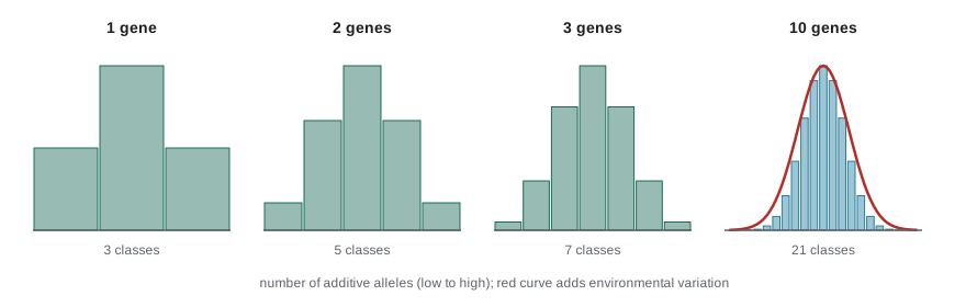
The general rule is that with n genes of equal additive effect, an F2 has 2n + 1 phenotypic classes and the fraction resembling either extreme parent is (1/4)ⁿ. If 1/256 of an F2 is as extreme as one parent, four genes are involved. Add environmental variation, which blurs the boundaries between classes, and the distribution becomes continuous.
Partitioning variation
Quantitative genetics describes variation with variances. The total phenotypic variance in a population, written V_P, can be divided into variance due to genetic differences (V_G) and variance due to environmental differences (V_E):
Genetic variance itself has components. Additive variance \(V_A\) comes from the average effects of alleles, which add up across loci. Dominance variance \(V_D\) comes from interactions between alleles at the same locus, and interaction variance \(V_I\) from interactions between loci (epistasis, lesson 5). The distinction matters because parents pass on alleles, not genotypes: a child receives one allele from each parent, so only the additive part of a parent's genetic value is reliably transmitted.
Heritability
Heritability measures how much of the variation in a trait, in a particular population and environment, is due to genetic differences. There are two versions:
| Measure | Definition | What it tells us |
|---|---|---|
| Broad-sense heritability, H² | V_G / V_P | The share of phenotypic variation due to all genetic differences |
| Narrow-sense heritability, h² | V_A / V_P | The share due to additive effects; predicts resemblance between relatives and response to selection |
Heritability is one of the most misunderstood ideas in biology. It describes variation in a population, not individuals: a heritability of 0.8 for height does not mean 80 per cent of a person's height is due to genes. It applies to a particular population in a particular environment and can change if either changes. And high heritability does not mean a trait cannot be changed by the environment. Height has a heritability of about 0.8 in well-nourished populations, yet average height rose by roughly 10 cm over the twentieth century in many countries because of better nutrition and health. The differences among individuals are largely genetic; the change in the average was environmental.
Estimating heritability
Heritability is estimated from the resemblance between relatives. The simplest method regresses offspring phenotypes on the average of their two parents (the midparent value). The slope of that regression estimates h². Twin studies compare identical (monozygotic) twins, who share all their genes, with fraternal (dizygotic) twins, who share half on average; the extra resemblance of identical twins indicates genetic influence. Today, genome-wide data on hundreds of thousands of people allow heritability to be estimated directly from DNA similarity among unrelated individuals.
import numpy as np
rng = np.random.default_rng(201)
# Simulate a trait with additive genes and environment, then estimate h2 from midparent regression
n_fam, loci = 2000, 100
h2_true = 0.6
def genotype(n):            # number of '+' alleles at each locus, frequency 0.5
    return rng.binomial(1, 0.5, size=(n, loci, 2))
mothers, fathers = genotype(n_fam), genotype(n_fam)
def breeding_value(g): return g.sum(axis=(1, 2)).astype(float)
va = breeding_value(mothers).var()
ve = va * (1 - h2_true) / h2_true
def phenotype(g): return breeding_value(g) + rng.normal(0, np.sqrt(ve), size=len(g))
# each child gets one random allele per locus from each parent
pick = lambda g: np.take_along_axis(g, rng.integers(0, 2, size=(n_fam, loci, 1)), axis=2)
child = np.concatenate([pick(mothers), pick(fathers)], axis=2)
mid = (phenotype(mothers) + phenotype(fathers)) / 2
kid = phenotype(child)
slope = np.polyfit(mid, kid, 1)[0]
print(f"true narrow-sense heritability: {h2_true}")
print(f"estimated from offspring-midparent regression slope: {slope:.2f}")true narrow-sense heritability: 0.6 estimated from offspring-midparent regression slope: 0.62
Response to selection: the breeder's equation
Breeders select the best individuals as parents, hoping to improve the next generation. How much improvement can they expect? The answer is the breeder's equation:
The selection differential \(S\) is how much the selected parents exceed the population mean; the response \(R\) is how much the offspring mean exceeds the original mean. Only the heritable share of the parents' advantage is passed on, so when \(h^2\) is low, even strong selection produces little response.
Worked problem
Predicting the response to selection
In a canola breeding program, the mean seed oil content is 44 per cent. Breeders select parent plants averaging 47 per cent. If the narrow-sense heritability of oil content is 0.5, what is the expected mean of the next generation?
Show solution
- S = 47 − 44 = 3 percentage points.
- R = h²S = 0.5 × 3 = 1.5 percentage points.
- Expected mean = 44 + 1.5 = 45.5 per cent.
- Repeated over many generations, such selection can produce large changes, as long as additive variance remains.
Answer: About 45.5 per cent oil. Canola itself is a product of this kind of selection: Canadian breeders at Agriculture Canada and the University of Manitoba developed it from rapeseed in the 1970s by selecting for low erucic acid and low glucosinolates.
Selection experiments show that most traits respond to selection, which demonstrates that they have additive genetic variance. The Illinois corn experiment, now running for more than 125 generations, has increased kernel oil content from about 5 per cent to over 20 per cent in the high line and reduced it to near zero in the low line. Dairy breeding provides another example: genomic selection, which predicts an animal's breeding value from DNA markers spread across the genome, has roughly doubled the rate of genetic improvement in milk yield in North American Holstein cattle since it was adopted around 2009.
Quantitative trait loci and polygenic scores
A quantitative trait locus (QTL) is a region of the genome containing one or more genes that affect a quantitative trait. QTLs are found by crossing lines that differ in a trait and testing which genetic markers (lesson 8) are associated with the trait in the offspring. In humans, genome-wide association studies (GWAS) test millions of variants in hundreds of thousands of people. Height, for example, has been linked to more than 12,000 variants, each with a tiny effect, which together explain a large share of its heritability. Combining these effects gives a polygenic score, an estimate of an individual's genetic predisposition. Polygenic scores are useful in research and are being tested in medicine, but they predict poorly in populations that differ in ancestry from the study participants, most of whom have been of European ancestry, raising important questions of equity. BIOL-410 returns to these methods.
Selection at a single locus
Population genetics asks how allele frequencies change. Consider selection against a recessive allele a with frequency q. If aa individuals do not reproduce at all (selection coefficient s = 1), the allele frequency in the next generation is
The second formula gives the frequency after t generations. Selection against a rare recessive is extremely slow, because almost all copies of a rare recessive allele are hidden in heterozygotes, where selection cannot see them. Reducing q from 0.01 to 0.005 takes 100 generations, about 2,500 years in humans. This is why proposals to eliminate recessive conditions by preventing affected people from reproducing, a goal of the eugenics movement (lesson 1), were biologically futile as well as unethical.
def generations_to_reach(q0, q_target, s=1.0):
    """Selection against a recessive (fitness of aa = 1 - s); iterate the exact recursion."""
    q, t = q0, 0
    while q > q_target:
        p = 1 - q
        mean_w = 1 - s * q * q
        q = (p * q + q * q * (1 - s)) / mean_w
        t += 1
    return t

for q0, qt in [(0.5, 0.25), (0.1, 0.05), (0.01, 0.005), (0.01, 0.001)]:
    t = generations_to_reach(q0, qt)
print(f"q from {q0} to {qt}: {t:5d} generations (about {25 * t:,} years at 25 years per generation)")q from 0.5 to 0.25: 3 generations (about 75 years at 25 years per generation) q from 0.1 to 0.05: 11 generations (about 275 years at 25 years per generation) q from 0.01 to 0.005: 100 generations (about 2,500 years at 25 years per generation) q from 0.01 to 0.001: 901 generations (about 22,525 years at 25 years per generation)
Mutation–selection balance
If harmful alleles are constantly removed by selection, why do they persist? Because new mutations keep creating them. An equilibrium is reached when the rate at which mutation creates harmful alleles equals the rate at which selection removes them. For a recessive allele with mutation rate μ and selection coefficient s against homozygotes, the equilibrium frequency is approximately
For a lethal recessive (s = 1) with a mutation rate of \(10^{-5}\) per generation, \(\hat{q} \approx \sqrt{10^{-5}} \approx 0.003\). For a dominant harmful allele the equilibrium is much lower, about \(\mu / s\), because heterozygotes are exposed to selection. Some recessive disease alleles are much more common than mutation–selection balance predicts. The sickle allele, for example, reaches frequencies of 10 to 20 per cent in parts of Africa because heterozygotes are protected against severe malaria, an example of heterozygote advantage that maintains the allele by balancing selection.
Inbreeding
Inbreeding, mating between relatives, increases homozygosity without directly changing allele frequencies. Its effect is measured by the inbreeding coefficient F, the probability that the two alleles at a locus in an individual are identical by descent, meaning both copies came from the same ancestral allele. The child of first cousins has F = 1/16. Inbreeding raises the frequency of homozygous recessive genotypes from q² to q² + Fpq, which for rare alleles is a large relative increase.
Worked problem
The effect of first-cousin marriage
A recessive condition has an allele frequency of q = 0.005. Compare the frequency of affected children from unrelated parents and from first cousins (F = 1/16).
Show solution
- Unrelated parents: q² = 0.005² = 0.000025, or 1 in 40,000.
- First cousins: q² + Fpq = 0.000025 + (1/16)(0.995)(0.005) = 0.000025 + 0.000311 = 0.000336, about 1 in 3,000.
- The risk is about 13 times higher for this rare allele.
- Overall, children of first cousins have roughly a 2 to 3 percentage point higher risk of a serious birth difference or genetic condition than the general population baseline of about 2 to 3 per cent.
Answer: About 1 in 40,000 versus about 1 in 3,000. The rarer the allele, the larger the relative effect of inbreeding, which is why rare recessive conditions are often found in children of related parents.
Inbreeding depression, the reduced survival and fertility of inbred offspring, is a major concern in conservation, where small populations cannot avoid mating between relatives, and in animal breeding, where popular sires can father thousands of offspring. In many cultures marriage between cousins is common, and genetic counselling and carrier screening can help such couples understand and manage their risks.
Common mistakes
MistakeA heritability of 0.8 means 80 per cent of each person’s trait is due to genes.
InsteadHeritability describes the share of variation in a population that is due to genetic differences, not a fraction of an individual.
MistakeA highly heritable trait cannot be changed by the environment.
InsteadHeight is highly heritable yet average height rose greatly with better nutrition.
MistakeStrong selection always produces a large response.
InsteadThe response depends on narrow-sense heritability: R = h²S; with low h², response is small.
MistakePreventing affected people from reproducing would quickly eliminate a recessive disease.
InsteadMost copies of rare recessive alleles are in healthy carriers, so selection against homozygotes is extremely slow.
MistakeInbreeding changes allele frequencies.
InsteadInbreeding increases homozygosity; it does not by itself change allele frequencies.
Summary and key terms
- Quantitative traits vary continuously because many genes of small additive effect and the environment contribute.
- With n additive genes, an F2 has 2n + 1 classes and (1/4)ⁿ resembles each extreme parent.
- Phenotypic variance divides into genetic (additive, dominance, interaction) and environmental components.
- Broad-sense heritability is V_G/V_P; narrow-sense heritability V_A/V_P predicts resemblance between relatives and response to selection.
- The breeder’s equation R = h²S predicts the response to selection.
- Selection against rare recessive alleles is very slow; mutation–selection balance keeps recessive alleles near √(μ/s).
- Inbreeding raises homozygote frequency to q² + Fpq; children of first cousins have F = 1/16.
- quantitative trait
- A trait that varies continuously and is influenced by many genes and the environment.
- polygenic
- Influenced by many genes.
- additive allele
- An allele that contributes a fixed amount to a quantitative trait.
- broad-sense heritability
- The proportion of phenotypic variance due to all genetic variance.
- narrow-sense heritability
- The proportion of phenotypic variance due to additive genetic variance.
- selection differential
- The difference between the mean of selected parents and the population mean.
- response to selection
- The change in mean phenotype in the offspring of selected parents.
- quantitative trait locus
- A genomic region containing genes that affect a quantitative trait.
- mutation–selection balance
- An equilibrium in which new harmful mutations are created as fast as selection removes them.
- inbreeding coefficient
- The probability that the two alleles at a locus are identical by descent.
Practice problems
Work each problem on paper first, then reveal the answer to check.
In an F2, 1/64 of plants resemble each parent. How many genes are involved?
Show answer
Three, since (1/4)³ = 1/64.
How many phenotypic classes are expected in an F2 for four additive genes?
Show answer
2 × 4 + 1 = 9.
If V_P = 50 and V_A = 20, what is h²?
Show answer
20/50 = 0.4.
A population has a mean of 100; selected parents average 110; h² = 0.3. Predict the offspring mean.
Show answer
R = 0.3 × 10 = 3, so the mean is 103.
Why can heritability differ between two populations for the same trait?
Show answer
Because it depends on the genetic and environmental variation present in each population.
What is the equilibrium frequency of a recessive lethal allele with μ = 4 × 10⁻⁶?
Show answer
√(4 × 10⁻⁶) = 0.002.
Why is selection against a rare recessive allele so slow?
Show answer
Most copies are in heterozygotes, which are not affected and are not selected against.
What is the inbreeding coefficient of a child of first cousins?
Show answer
1/16.
With q = 0.01 and F = 1/16, what is the frequency of aa?
Show answer
q² + Fpq = 0.0001 + 0.0625 × 0.99 × 0.01 ≈ 0.00072.
Give an example of heterozygote advantage.
Show answer
Sickle-cell heterozygotes are protected against severe malaria.
Lesson quiz · 5 questions
Score 60% or more to complete this lesson.
Create a free account to save your progress, take quizzes and earn a certificate.