
BIOL-107 · Lesson 4 of 12 · 27 min
Studying cells: microscopy and laboratory methods
Almost everything we know about cells came from a new way of seeing or measuring them. Hooke needed a lens to see cork cells; the structure of the mitochondrion waited for the electron microscope; the shapes of thousands of proteins came from X-ray crystallography and, more recently, cryo-electron microscopy. This lesson introduces the main tools of cell biology, the arithmetic behind them, and the safety rules that apply in any laboratory that handles cells.
Size scales in biology
Cell biology spans a huge range of sizes, and the units change as you go down. A millimetre (mm) is a thousandth of a metre; a micrometre (µm) is a thousandth of a millimetre; a nanometre (nm) is a thousandth of a micrometre. Most cells are measured in micrometres, and most of their molecules in nanometres.
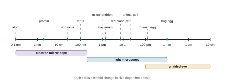
| Object | Typical size | Can be seen with |
|---|---|---|
| Frog egg | About 1 mm | Unaided eye |
| Human egg cell | About 120 µm | Unaided eye, just |
| Typical animal cell | About 10 to 30 µm | Light microscope |
| Red blood cell | About 7 to 8 µm | Light microscope |
| Bacterium (E. coli) | About 1 × 2 µm | Light microscope |
| Mitochondrion | About 0.5 to 1 µm wide | Light microscope (barely); detail needs electron microscope |
| Virus (influenza) | About 100 nm | Electron microscope |
| Ribosome | About 25 nm | Electron microscope |
| Membrane thickness | About 7 to 10 nm | Electron microscope |
| Protein (hemoglobin) | About 5 nm | Electron microscope, X-ray crystallography |
Magnification and resolution
A microscope does two things. It magnifies, making the image larger, and it resolves, making separate objects appear separate. Magnification without resolution is useless: blowing up a blurry photograph only gives a bigger blur. Resolution is the smallest distance between two points that can still be told apart.
In a compound light microscope, the total magnification is the product of the objective lens and the eyepiece (ocular) magnifications. A 40× objective with a 10× eyepiece gives 400×. The resolution, though, is set by the wavelength of light and the light-gathering ability of the objective, measured by its numerical aperture (NA). Ernst Abbe showed in the 1870s that the smallest resolvable distance is roughly:
Here \(\lambda\) is the wavelength of light and NA is typically 0.1 for a low-power objective and up to about 1.4 for an oil-immersion lens, which uses a drop of oil between lens and slide to collect more light. With green light at 550 nm and an NA of 1.4, \(d \approx 550/2.8 \approx 200\) nm. That is the famous limit of the light microscope: about 0.2 µm. Objects closer together than that blur into one.
# Abbe resolution limit d = wavelength / (2 * NA)
def abbe_nm(wavelength_nm, na):
    return wavelength_nm / (2 * na)

for name, lam, na in [("10x objective, green light", 550, 0.25),
                      ("40x objective, green light", 550, 0.65),
                      ("100x oil immersion, green", 550, 1.40),
                      ("100x oil immersion, blue", 450, 1.40)]:
    print(f"{name:<29} d = {abbe_nm(lam, na):6.0f} nm")

# Electron beam: wavelength about 0.0025 nm at 200 kV, but lenses are imperfect
print("Theoretical electron limit at NA 0.01:", round(abbe_nm(0.0025, 0.01), 3), "nm")10x objective, green light d = 1100 nm 40x objective, green light d = 423 nm 100x oil immersion, green d = 196 nm 100x oil immersion, blue d = 161 nm Theoretical electron limit at NA 0.01: 0.125 nm
Electrons behave as waves with wavelengths thousands of times shorter than visible light, so electron microscopes can in principle resolve far smaller objects. In practice, imperfect magnetic lenses and damage to the specimen limit biological samples to roughly 0.1 to a few nanometres, depending on the method. That is still a thousand times better than light.
Measuring cells: scale bars and calibration
Micrographs in papers carry a scale bar rather than a magnification, because images are resized when printed or viewed on screens. To measure an object, compare it with the scale bar. In the laboratory, the eyepiece contains a reticle (a small ruler) whose divisions are calibrated against a stage micrometer, a slide with a ruled scale of known spacing, for each objective.
Worked problem
Using a scale bar
On a printed micrograph, a scale bar labelled 10 µm is 25 mm long. A cell in the same image measures 62 mm across. How big is the cell, and what is the magnification of the printed image?
Show solution
- Find the image scale: 25 mm on paper represents 10 µm, so 1 mm on paper is 0.4 µm.
- Cell size = 62 mm × 0.4 µm per mm = 24.8 µm.
- Magnification = image size ÷ actual size. Convert to the same unit: 25 mm = 25,000 µm.
- Magnification = 25,000 µm ÷ 10 µm = 2,500×.
Answer: The cell is about 25 µm across, and the printed image is magnified about 2,500 times.
# Calibrating an eyepiece reticle with a stage micrometer
stage_div_um = 10          # one stage micrometer division = 10 um
# Observed: 40 eyepiece divisions line up with 13 stage divisions at 40x
eyepiece_divs, stage_divs = 40, 13
um_per_eyepiece_div = stage_divs * stage_div_um / eyepiece_divs
print("One eyepiece division =", um_per_eyepiece_div, "um at 40x")

cells = [7.5, 8.0, 6.5, 7.0, 8.5]      # eyepiece divisions across five cells
sizes = [c * um_per_eyepiece_div for c in cells]
print("Cell diameters (um):", [round(s, 2) for s in sizes])
print("Mean diameter:", round(sum(sizes) / len(sizes), 2), "um")One eyepiece division = 3.25 um at 40x Cell diameters (um): [24.38, 26.0, 21.12, 22.75, 27.62] Mean diameter: 24.38 um
Kinds of light microscopy
Cells are mostly water and are nearly transparent, so ordinary bright-field microscopy shows little unless cells are stained, which usually kills them. Several techniques overcome this:
| Technique | How it creates contrast | Typical use | Live cells? |
|---|---|---|---|
| Bright-field | Absorption of light, often after staining with dyes | Stained tissue sections, Gram-stained bacteria | Usually no (stains kill) |
| Phase contrast and DIC | Converts small differences in refractive index into brightness differences | Watching living cells divide or move in culture | Yes |
| Fluorescence | Molecules absorb light of one colour and emit another; filters show only the emitted light | Locating specific proteins, DNA or organelles | Yes, with suitable labels |
| Confocal | Laser scanning with a pinhole rejects out-of-focus light, giving thin optical sections | 3-D images of cells and tissues | Yes |
| Super-resolution (STED, PALM, STORM) | Tricks with fluorescence that beat the Abbe limit, down to about 20 nm | Fine structure of synapses, cytoskeleton, membrane domains | Often |
Fluorescence microscopy transformed cell biology. Antibodies can be tagged with fluorescent dyes to show where a protein sits in fixed cells (immunofluorescence). Even better, scientists can fuse the gene for green fluorescent protein (GFP), originally from a jellyfish, to the gene for a protein of interest, so living cells make their own glowing tag. Osamu Shimomura, Martin Chalfie and Roger Tsien shared the 2008 Nobel Prize in Chemistry for GFP, and Eric Betzig, Stefan Hell and William Moerner shared the 2014 prize for super-resolution fluorescence microscopy.
Electron microscopy
Electron microscopes use beams of electrons focused by magnetic lenses in a vacuum. A transmission electron microscope (TEM) passes electrons through a very thin section of a specimen, typically 50 to 100 nm thick, stained with heavy metals that scatter electrons. It shows internal structure: membranes, ribosomes, the folds inside mitochondria. A scanning electron microscope (SEM) sweeps a beam across a specimen coated with a thin metal layer and detects electrons bounced off the surface, producing detailed three-dimensional-looking images of surfaces.
Classical electron microscopy has drawbacks. Samples must be fixed, dehydrated, sliced and stained, so cells are dead, and preparation can create artefacts. Cryo-electron microscopy (cryo-EM) avoids much of this: samples are frozen so quickly that water forms glass-like ice instead of crystals, preserving molecules in a near-natural state. Computers combine tens of thousands of images of individual molecules to reconstruct their 3-D shapes, now often at near-atomic resolution. Jacques Dubochet, Joachim Frank and Richard Henderson shared the 2017 Nobel Prize in Chemistry for developing it.
| Feature | Light microscope | Transmission EM | Scanning EM |
|---|---|---|---|
| Radiation | Visible light | Electrons through the sample | Electrons off the surface |
| Best resolution (biological) | About 200 nm (about 20 nm with super-resolution) | About 0.1 to 2 nm | About 1 to 10 nm |
| Live specimens | Yes | No | No |
| Colour | True colour or fluorescent labels | Greyscale (false colour added) | Greyscale (false colour added) |
| Typical image | Whole cells, tissues | Internal structures, organelles | Surfaces of cells and organisms |
Taking cells apart: fractionation and biochemistry
Microscopes show where things are; biochemistry shows what they do. To study an organelle, biologists break cells open gently (homogenization) and separate the parts by spinning them in a centrifuge. In differential centrifugation, the homogenate is spun at increasing speeds: nuclei and large debris pellet first, then mitochondria (and in plants, chloroplasts), then smaller membrane fragments and ribosomes. Each pellet can then be tested for enzymes and other molecules.
Centrifuge speeds are given as relative centrifugal force (RCF), a multiple of Earth's gravity (g), rather than revolutions per minute, because the force depends on the radius of the rotor: \(\text{RCF} = 1.118 \times 10^{-5} \times r \times \text{rpm}^2\), with \(r\) in centimetres.
import math
# Relative centrifugal force from rotor radius (cm) and speed (rpm)
def rcf(radius_cm, rpm):
    return 1.118e-5 * radius_cm * rpm ** 2

def rpm_for(radius_cm, target_g):
    return math.sqrt(target_g / (1.118e-5 * radius_cm))

print("Microcentrifuge, r = 7.5 cm, 13,000 rpm:", round(rcf(7.5, 13000)), "x g")
print("Speed for 600 x g at r = 15 cm:", round(rpm_for(15, 600)), "rpm")
print("Speed for 100,000 x g at r = 8 cm:", round(rpm_for(8, 100000)), "rpm")Microcentrifuge, r = 7.5 cm, 13,000 rpm: 14171 x g Speed for 600 x g at r = 15 cm: 1892 rpm Speed for 100,000 x g at r = 8 cm: 33438 rpm
Other basic methods appear throughout biology and will recur in later courses. Gel electrophoresis separates proteins or DNA fragments by size as they move through a gel in an electric field; smaller molecules move faster. Spectrophotometry measures how much light a solution absorbs, which gives concentrations of DNA, proteins or pigments. Cell culture grows animal or plant cells in flasks with nutrients, at controlled temperature (37 °C for human cells) and carbon dioxide levels. Flow cytometry counts thousands of individual cells per second as they pass a laser, measuring size and fluorescent labels.
Working safely in a cell biology laboratory
Laboratories that handle chemicals and living cells follow two sets of rules: chemical hazard communication and biosafety. You will use both from the first lab session. HSE-102 covers hazard communication in detail; here is what a biology student needs first.
Chemical hazards in Canadian workplaces, including teaching and research labs, fall under WHMIS (the Workplace Hazardous Materials Information System), aligned with the international Globally Harmonized System (GHS). Products carry supplier labels with pictograms, and every hazardous product has a safety data sheet (SDS) describing its hazards, handling and first aid. Biosafety is governed federally by the Human Pathogens and Toxins Act and its regulations, administered by the Public Health Agency of Canada (PHAC). Work with Risk Group 2 or higher human pathogens or toxins needs a PHAC licence, and facilities must meet the Canadian Biosafety Standard (third edition, 2022), which sets physical and operational requirements for containment levels 1 to 4.
| Level | Typical agents | Key practices and equipment |
|---|---|---|
| Level 1 | Organisms not known to cause disease in healthy adults, such as non-pathogenic E. coli K-12 and baker’s yeast | Good microbiological practice, hand washing, lab coat, no eating or drinking |
| Level 2 | Agents of moderate risk, such as Staphylococcus aureus and human cell lines | Restricted access, biological safety cabinet for aerosol-producing work, eye protection, decontamination of waste |
| Level 3 | Serious airborne pathogens, such as Mycobacterium tuberculosis | Controlled access, directional airflow, respirators, all work in safety cabinets |
| Level 4 | Dangerous agents with no treatment, such as Ebola virus | Positive-pressure suits or cabinet lines, isolated building systems |
In Canada these are called containment levels (CL1 to CL4); the agents are classified into risk groups (RG1 to RG4). Undergraduate teaching labs normally work at CL1, and sometimes CL2 for human cells or common bacteria.
A few rules apply in every biology lab regardless of level: know where the eyewash, safety shower and spill kit are; wear a lab coat, closed shoes and eye protection; never pipette by mouth; keep food and drink out; wash hands before leaving; dispose of sharps, chemicals and biological waste in the correct containers; and report every spill or injury, however small. Most laboratory incidents involve ordinary hazards such as broken glass, hot plates and chemical splashes rather than exotic microbes.
Common mistakes
MistakeHigher magnification always means more detail.
InsteadDetail depends on resolution; past the resolution limit, extra magnification only enlarges blur (empty magnification).
MistakeElectron microscopes show cells in colour.
InsteadElectron images are greyscale; colours in published images are added afterwards (false colour).
MistakeA 100× objective with a 10× eyepiece gives 110× magnification.
InsteadTotal magnification is the product, 100 × 10 = 1,000×.
MistakeCentrifuge settings in rpm are the same on every machine.
InsteadThe force depends on rotor radius; protocols give relative centrifugal force (× g) so they work on any centrifuge.
MistakeBiosafety rules only matter in labs with dangerous pathogens.
InsteadBasic practices apply at every level, and human cell lines are usually handled at level 2 because they may carry unknown agents.
Summary and key terms
- Cells are measured in micrometres and molecules in nanometres; most cells are too small to see without a microscope.
- Magnification enlarges an image; resolution separates close objects. Light microscopes are limited to about 200 nm by the Abbe limit d = λ/(2 NA).
- Scale bars and calibrated reticles let you measure cells: size = image length × (actual length of scale bar ÷ image length of scale bar).
- Phase contrast, fluorescence, confocal and super-resolution microscopy reveal living cells and specific molecules; GFP tags proteins in live cells.
- Transmission and scanning electron microscopes resolve nanometre detail in dead, prepared specimens; cryo-EM reveals molecular structures.
- Differential centrifugation separates organelles by size and density; forces are given in × g.
- Labs follow chemical hazard communication (GHS labels and SDSs) and biosafety containment levels 1 to 4.
- micrometre
- One millionth of a metre (µm); the usual unit for cell sizes.
- resolution
- The smallest distance at which two points can still be distinguished as separate.
- numerical aperture
- A measure of how much light an objective lens can collect; higher values give better resolution.
- scale bar
- A line on a micrograph labelled with the real distance it represents.
- fluorescence microscopy
- Microscopy that detects light emitted by fluorescent molecules to show specific structures.
- green fluorescent protein
- A jellyfish protein that glows green and can be fused to other proteins to track them in living cells.
- transmission electron microscope
- An electron microscope that passes electrons through thin sections to show internal structure.
- cryo-electron microscopy
- Electron microscopy of rapidly frozen samples, used to determine the 3-D structures of molecules.
- differential centrifugation
- Separating cell components by spinning them at increasing speeds.
- containment level
- A set of facility and practice requirements matched to the risk of the biological agents handled.
Practice problems
Work each problem on paper first, then reveal the answer to check.
A microscope has a 40× objective and a 15× eyepiece. What is the total magnification?
Show answer
600×.
Calculate the Abbe resolution limit for blue light (450 nm) with an objective of NA 0.95.
Show answer
d = 450 / (2 × 0.95) ≈ 237 nm.
Why can a light microscope not show the internal structure of a ribosome?
Show answer
A ribosome is about 25 nm, far below the light microscope’s resolution of about 200 nm.
A 5 µm scale bar is 20 mm long on a printout, and a bacterium is 8 mm long. How long is the bacterium?
Show answer
8 × (5/20) = 2 µm.
Name a technique for watching living, unstained cells divide.
Show answer
Phase contrast or differential interference contrast (DIC) microscopy, or fluorescence with live-cell labels.
How does GFP let biologists track a protein in living cells?
Show answer
The GFP gene is fused to the protein’s gene, so the cell makes the protein with a fluorescent tag attached.
Give one advantage and one limitation of transmission electron microscopy.
Show answer
Advantage: nanometre resolution of internal structures. Limitation: samples must be dead, thin and stained, risking artefacts.
In differential centrifugation, which fraction pellets first, and why?
Show answer
Nuclei, because they are the largest and densest organelles and sediment at low force.
Calculate the RCF for a rotor of radius 10 cm spinning at 3,000 rpm.
Show answer
1.118 × 10^−5 × 10 × 3000² ≈ 1,006 × g.
At what containment or biosafety level are human cell lines usually handled, and why?
Show answer
Level 2, because human cells may carry unknown viruses or other agents.
Lesson quiz · 5 questions
Score 60% or more to complete this lesson.
Create a free account to save your progress, take quizzes and earn a certificate.