Energy modelling principles

For the third seminar Holm brings a cardboard box, a thermometer, a desk lamp and a brick. He puts the thermometer and the brick in the box, closes it, and switches on the lamp above it. 'Everything an energy simulation does,' he says, 'is a careful version of what happens in this box. Heat comes in through the lid from the lamp. Heat leaks out through the walls. Some of it is stored in the air and some in the brick. The temperature inside depends on how fast each of those happens, hour by hour.' Joon-ho asks how many equations EnergyPlus solves for the hub. 'Tens of thousands each time step. But each one says the same thing as this box: what comes in, minus what goes out, equals what is stored.'

The heat balance

At the heart of every whole-building energy model is a balance of energy, written for each surface and for the air of each thermal zone at every time step. For the air of a zone, the heat added by convection from the surfaces, by internal gains from people, lights and equipment, by air entering from outside or from other zones, and by the heating or cooling system must equal the rate at which the air's heat content changes.

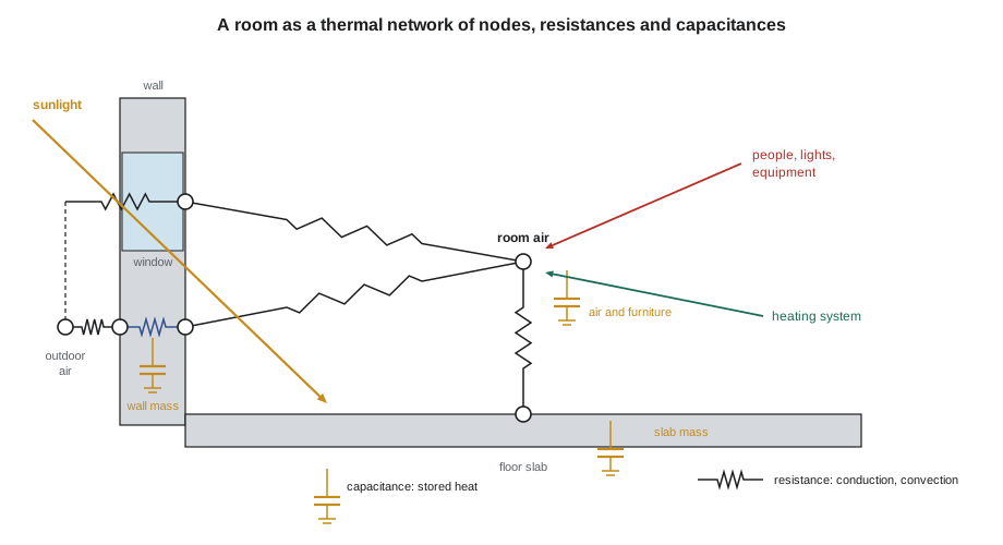
Each surface has its own balance. On its outside face, sunlight absorbed, long-wave radiation exchanged with the sky and the ground, and convection with the outside air balance the heat conducted into the wall. On its inside face, conduction from within the wall balances convection to the room air, long-wave radiation exchanged with the other surfaces of the room, and the share of sunlight, lights and people's radiant heat that lands on it. Inside the wall, heat conducts through the layers and is stored in their mass, which delays and smooths the flow. EnergyPlus calls this method the heat balance method; it is the approach recommended in ASHRAE's Handbook of Fundamentals and the one most modern engines use.

Resistances and capacitances

Holm likes to draw energy models as electrical networks, because the analogy is exact. Temperature is like voltage, heat flow like current, thermal resistance like electrical resistance, and the heat stored in a material like the charge stored in a capacitor. A wall of high thermal resistance is a large resistor; a concrete slab is a large capacitor. The time constant of a part of the building, its capacitance multiplied by the resistance through which it gains or loses heat, measures how quickly it responds.

A light building with a time constant of a few hours follows the outdoor temperature and the sun closely: it heats up quickly on a sunny afternoon and cools quickly at night. A heavy, well-insulated building with a time constant of several days barely notices a single cold night. Neither is better in itself. Light buildings respond quickly to their heating system, which saves energy in buildings used intermittently; heavy buildings store solar gain and ride through outages and heat waves, which matters for resilience.

The students build the simplest useful energy model: the whole hub as a single zone with one resistance, its total conductance, and one capacitance, the heat stored in its air, furniture and exposed structure. They step it through a clear, cold week hour by hour, with sunlight through the south windows, internal gains during opening hours and a heating system that holds the setpoint. Then they repeat the week with a two-day power failure, comparing a light timber interior with an exposed concrete slab.

# The whole hub treated as one thermal zone as a resistance-capacitance network, stepped hour by hour through a cold, clear week
import math
UA = 1150.0            # envelope and ventilation conductance after heat recovery, W/K
SET = 20.0             # heating setpoint, C
def week(cap_kj_per_k, outage):
    t_in = SET; energy = 0.0; low = 99.0
    for h in range(168):
        hour = h % 24
        heat_on = not (outage and 48 <= h < 96)   # a two-day power failure from Wednesday midnight
        t_out = -18.0 - 6.0 * math.cos(2 * math.pi * (hour - 4) / 24)
        sun = max(0.0, math.sin(math.pi * (hour - 8) / 9)) * 38000.0 if 8 <= hour <= 17 else 0.0   # solar gain, W
        people = 12000.0 if (8 <= hour < 21 and h < 120) else 1500.0                            # people, lights, equipment, W
        for _ in range(6):                               # ten-minute sub-steps for stability
            q_loss = UA * (t_in - t_out)
            q_heat = 0.0
            if heat_on:
                need = q_loss - sun - people + (SET - t_in) * cap_kj_per_k * 1000 / 600
                q_heat = min(max(need, 0.0), 120000.0)   # plant capacity 120 kW
            t_in += (sun + people + q_heat - q_loss) * 600 / (cap_kj_per_k * 1000)
            energy += q_heat * 600 / 3.6e6               # kWh
        if not heat_on:
            low = min(low, t_in)
    return energy, low
for name, cap in (("light timber interior", 60000.0), ("exposed concrete slab", 240000.0)):
    e, _ = week(cap, False)
    _, lo = week(cap, True)
    tau = cap * 1000 / UA / 3600
    print(f"{name:22s} time constant {tau:5.1f} h; heating {e * 1:6.0f} kWh per week; lowest during outage {lo * 1 + 0:5.1f} C")

light timber interior  time constant  14.5 h; heating   4931 kWh per week; lowest during outage  -8.4 C
exposed concrete slab  time constant  58.0 h; heating   4908 kWh per week; lowest during outage   6.9 C

The result surprises the students. With the heating on, the heavy and light interiors use almost exactly the same heating energy over the week, about 4,900 kWh, because in a cold Prairie week the hub needs heat nearly all the time and the slab has little chance to store useful surplus. During the outage, though, the difference is dramatic: the light interior falls to about −8 °C, while the slab keeps the hub at about 7 °C. The time constant explains why: about 14 hours for the light interior and 58 for the slab. Thermal mass changes resilience far more than it changes annual energy in this climate, a conclusion Holm wants them to test with the full model rather than take from the simple one.

Time steps and solution methods

A simulation advances in time steps. EnergyPlus typically uses steps of 10 to 15 minutes for the zone heat balance and may take shorter steps for HVAC systems when conditions change quickly. Short steps are more accurate but slower; steps that are too long can make the calculation unstable, which is why the students' program divides each hour into six sub-steps. Conduction through walls is calculated with methods that account for the delay caused by stored heat: EnergyPlus uses conduction transfer functions by default and a finite difference method when materials change properties, for example phase change materials.

Most engines solve the zones and the systems in sequence at each step: first the loads on each zone, then the response of the systems serving them, then a correction to the zone temperatures if the systems could not meet the load. This is why an undersized system in a model shows up as unmet hours, the number of occupied hours in which a zone's temperature falls outside its setpoint band. Codes and rating systems limit unmet hours, often to a few hundred a year, as a check that the modelled systems can actually do their job.

Inputs: what the model needs

A whole-building energy model needs six kinds of input, and Holm insists that the students keep a written record of every one, with its source.

• Weather: the hourly file for the question being asked, as in Lesson 2.
• Geometry: the shape of the building, its zones and its surfaces, including windows and shading, as in Lesson 4.
• Constructions: the layers of every wall, roof, floor and window, with conductivity, density, specific heat and optical properties.
• Internal loads: people, lighting and equipment, as densities and with schedules that say when they occur.
• Air flows: infiltration through the envelope, ventilation for occupants and any natural ventilation.
• Systems: the heating, cooling, ventilation and hot water equipment, its controls and its performance curves.

Each input is uncertain to a different degree. The geometry is usually known well; the conductivity of mineral wool is known well; the number of people in the hall on a Saturday evening, the plug loads of a daycare and the way occupants will open windows are known poorly. Lesson 5 shows how to find out which uncertainties matter.

Schedules and people

Schedules tell the model when things happen. A schedule might say that the reading room's lights are at full power from 9 a.m. to 9 p.m. on weekdays, at 0.3 of full power on Sunday, and off otherwise; that the hall holds 300 people on two evenings a week; that the heating setpoint drops at night. Default schedules supplied with software and standards, such as those in the NECB, are designed for compliance, so that every building is judged on the same assumptions, not for prediction. A model built for compliance with standard schedules may differ greatly from how the building is actually used.

Sethi tells the students that schedules are where most models go wrong. On a library she modelled, the standard schedule assumed the building closed at 6 p.m.; in reality it ran homework programs until 9 p.m. and rented its meeting rooms on weekends, and the measured energy use was a third higher than the model. 'Ask the client how the building will really be used. Write it down. Then ask the people who will run it, because they will tell you something different.'

Systems and plant

The heating and cooling systems are modelled with performance curves that describe how their capacity and efficiency change with conditions. An air-source heat pump's heating capacity and coefficient of performance (COP) fall as the outdoor temperature drops; a model that uses a single rated COP will badly overestimate its winter performance in Winnipeg. The students met this in Environmental Systems II, where the hub's heat pumps stopped below −30 °C (−22 °F) and backup heat carried the coldest night. In the full model, the heat pump's curves come from the manufacturer's data at several temperatures, and the backup heat is modelled explicitly.

Systems also have controls, which are often more important than the equipment. A heat recovery ventilator that bypasses its core in mild weather, a demand-controlled ventilation system that reduces outdoor air when carbon dioxide levels are low, and night setback of the heating setpoint all change energy use substantially. Models should represent the controls the building will actually have, and the commissioning process should check that the real controls match the model.

From loads to energy to carbon

The model produces hourly energy use for each end use: space heating, cooling, fans, pumps, lighting, equipment and hot water. Summed over the year and divided by floor area, these give the energy use intensity. Multiplied by emission factors, as in Sustainable and Regenerative Design, they give operational emissions. Holm reminds the students that the emission factor should match the hour as well as the place where it matters: on Manitoba's hydro grid the annual average is adequate, because every hour is nearly carbon-free.

Checking the model

Before trusting any result, the modeller checks the model. Holm gives the students a list they will use for the rest of the course.

• Look at the geometry in three dimensions: are windows on the right faces, are surfaces facing the right way, are any missing?
• Check the area, volume and window share against the drawings.
• Compare the design heating load with a hand calculation of conductance times temperature difference.
• Plot a winter week and a summer week of zone temperatures, loads and system output; do they make physical sense?
• Check unmet hours and find out where and when they occur.
• Compare the EUI and the end-use split with benchmarks for similar buildings.
• Change one input by a known amount and check that the result moves in the expected direction and by a plausible amount.

Exercise 3: a first whole-building model

Using the class's chosen tool, each student builds a first energy model of the hub with a single zone per floor.

• Record every input and its source in an input log.
• Run a typical year and report EUI and end uses.
• Check the design heating load against a hand calculation.
• Plot a winter and a summer week and explain what you see.

Self-critique checklist

• Have I logged every input and its source?
• Does every major result pass a hand check?
• Are my schedules realistic for the building's real use?
• Do my heat pump curves cover the full range of outdoor temperature?