Whole-building life cycle assessment

Mei Takahashi, the life cycle assessment consultant who guided the students through their first whole-building LCA in Sustainable and Regenerative Design, returns for the tenth seminar with a spreadsheet of more than four hundred rows. It is the bill of materials for the hub's current design, every item from the piles to the roof membrane, with a quantity, a unit, an environmental product declaration or a generic data source, and a result in kilograms of carbon dioxide equivalent. At the bottom is a single number: about 190 kg CO₂e per square metre of upfront carbon. 'You calculated this last year,' she says. 'Today I want you to ask how wrong it could be, and whether that matters.'

Whole-building LCA in brief

A whole-building life cycle assessment estimates the environmental impacts of a building over its whole life, from the extraction of raw materials to demolition and beyond. The European standard EN 15978 divides the life into modules: A1 to A3, the product stage (raw materials, transport to the factory, manufacturing); A4 and A5, transport to site and construction; B1 to B7, the use stage, including maintenance, repair, replacement and refurbishment (B2 to B5) and operational energy and water (B6 and B7); C1 to C4, the end of life (demolition, transport, waste processing, disposal); and module D, the benefits and loads beyond the system boundary, such as the reuse or recycling of materials. Upfront carbon is the sum of A1 to A5; embodied carbon includes the A, B1 to B5 and C modules; whole-life carbon adds operational carbon from B6 and B7.

Environmental product declarations (EPDs) report the impacts of specific products, verified by a third party under standards such as ISO 14025, ISO 21930 for construction products and EN 15804. Where no EPD exists, the analyst uses industry-average EPDs or generic data from databases. The students learned that biogenic carbon, the carbon stored in wood and other bio-based materials, must be reported separately from fossil emissions, because it returns to the atmosphere if the material burns or decays.

Tools and data

Whole-building LCA tools combine a bill of materials with a database of impacts. In Canada the most widely used free tool is the Athena Impact Estimator for Buildings, developed by the Athena Sustainable Materials Institute; commercial tools such as One Click LCA and the Building Transparency organization's EC3 tool for comparing EPDs are also common. The National Research Council has published national guidelines for whole-building LCA to make Canadian assessments consistent. BIM-integrated tools take quantities directly from the model, which saves effort but inherits every error in the model's quantities and classification.

Takahashi's first lesson is that the bill of materials matters more than the tool. Errors in quantities, such as a concrete slab counted twice or rebar left out, and in the choice of data, such as a generic value for an unusually carbon-intensive product, change results far more than differences between tools. She checks every LCA with three questions: do the largest items make sense for this building, do the quantities reconcile with the structural and architectural drawings, and does the result fall in the range of published benchmarks for similar buildings?

Sources of uncertainty

LCA results carry several kinds of uncertainty. Takahashi divides them into four.

• Data uncertainty: the impact per unit of a product varies between manufacturers, plants and years. A generic value for concrete may differ from the actual mix by a large margin; an EPD for a specific product is more certain but still has a stated variability.
• Quantity uncertainty: at the design stage the quantities are estimates, and they change as the design develops; contingencies, waste and items left out add to the error.
• Scenario uncertainty: the use stage and end of life depend on assumptions about replacement intervals, refurbishment, demolition practice and future recycling, decades away.
• Methodological choices: the boundary of the study, the treatment of biogenic carbon, the allocation of impacts to recycled content, and the choice of a 50 or 60 year study period.

Each can be explored. Data and quantity uncertainty lend themselves to Monte Carlo simulation, in which the analyst assigns each uncertain value a probability distribution and samples the whole calculation thousands of times. Scenario and methodological uncertainty are better explored with alternative scenarios, each stated clearly.

Monte Carlo analysis

In a Monte Carlo analysis, each uncertain input is drawn at random from its distribution, the result is calculated, and the process is repeated many times. The collection of results approximates the distribution of the output, from which the analyst reports a median and a range, such as the values below which 5 and 95 in 100 of the results fall. Triangular distributions, defined by a low, most likely and high value, are convenient when the analyst has only rough knowledge; where data allow, lognormal distributions often fit the skewed spread of impact factors better.

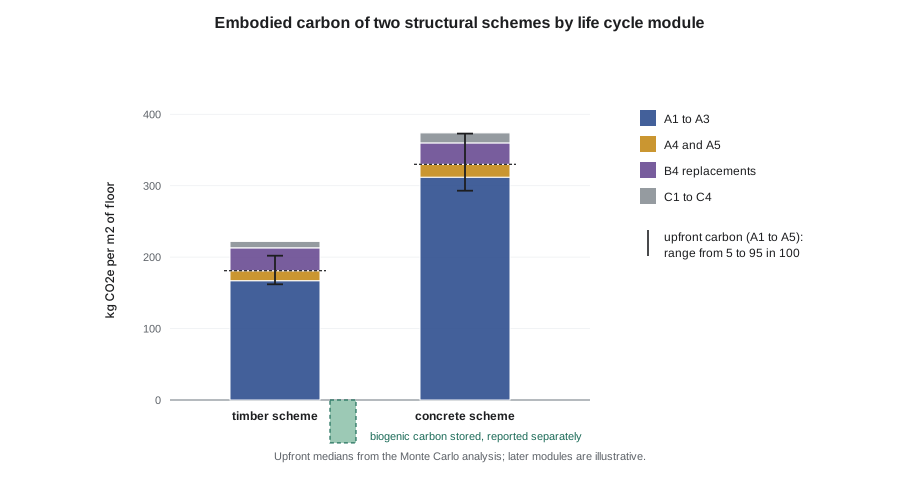
The students apply Monte Carlo analysis to the upfront carbon of the hub's two structural schemes from second year: the timber scheme they chose, with CLT and glulam on concrete foundations, and the concrete frame they rejected. Then they ask a sharper question: does switching the timber scheme's foundation concrete to a lower-carbon mix reliably reduce its carbon?

# Upfront carbon of two structural schemes for the hub, with uncertainty, by Monte Carlo sampling
import random
random.seed(10)
AREA = 2458.0
def tri(lo, mode, hi):
    return random.triangular(lo, hi, mode)
def timber(conc_mode=290):
    clt = 610.0 * tri(95, 125, 180)         # m3 of CLT and glulam x kg CO2e per m3 (fossil, cradle to gate)
    conc = 520.0 * tri(conc_mode - 60, conc_mode, conc_mode + 90)   # m3 of foundations and slab on grade
    steel = 38000.0 * tri(0.9, 1.3, 2.0)     # kg of connectors and steel
    envelope = AREA * tri(45, 60, 85)        # per m2 of floor
    return clt + conc + steel + envelope
def concrete():
    conc = 1450.0 * tri(230, 300, 400)
    rebar = 140000.0 * tri(0.6, 0.9, 1.4)
    steel = 52000.0 * tri(0.9, 1.3, 2.0)
    envelope = AREA * tri(45, 60, 85)
    return conc + rebar + steel + envelope
N = 5000
t = sorted(timber() / AREA for _ in range(N))
c = sorted(concrete() / AREA for _ in range(N))
pairs = sum(1 for _ in range(N) if timber() < concrete())
def p(v, q):
    return v[int(q * (len(v) - 1))]
for name, v in (("timber scheme", t), ("concrete scheme", c)):
    print(f"{name:16s} median {p(v, 0.5) * 1:5.1f} kg CO2e/m2, 90 in 100 range {p(v, 0.05) * 1:5.1f} to {p(v, 0.95) * 1:5.1f}")
print(f"timber lower than concrete in {pairs} of {N} draws")
low = sum(1 for _ in range(N) if timber(220) < timber(290))
print(f"low-carbon mix lowers the timber scheme in {low} of {N} draws")

timber scheme    median 181.1 kg CO2e/m2, 90 in 100 range 162.2 to 201.5
concrete scheme  median 330.1 kg CO2e/m2, 90 in 100 range 292.7 to 372.8
timber lower than concrete in 5000 of 5000 draws
low-carbon mix lowers the timber scheme in 4106 of 5000 draws

The timber scheme's upfront carbon has a median of about 181 kg CO₂e/m², with a 90 in 100 range of about 162 to 202; the concrete scheme's median is about 330, with a range of about 293 to 373. The ranges do not overlap, and the timber scheme is lower in every one of 5,000 draws: the choice between the schemes is robust to the uncertainty. The low-carbon mix is a different story. It lowers the timber scheme's carbon in only about 4,100 of 5,000 draws, about 82 in 100. That is still a good bet, but the result is no longer certain.

Takahashi points out a weakness in the students' program that also explains part of that uncertainty. The program draws the envelope's carbon independently for each scheme, as if the two schemes had different, unrelated envelopes. In reality the envelopes are the same; their uncertainty affects both schemes equally and cancels when they are compared. A careful comparison draws shared items once and applies them to both options, so that only the differences carry uncertainty into the comparison. Correlation between inputs matters as much as their spread.

Scenarios for the use stage and end of life

For the parts of the life cycle that lie decades ahead, scenarios are more honest than probability distributions. Takahashi asks the students to test three questions with alternative scenarios.

• Replacements: how often will the roof membrane, the windows, the heat pumps and the solar panels be replaced over sixty years? Replacing photovoltaic panels twice, rather than once, adds noticeably to the hub's embodied carbon.
• Refrigerants: how much refrigerant will leak from the heat pumps over their life, and what is its global warming potential? Refrigerant leakage can rival the embodied carbon of the equipment itself, which is why the hub's design specifies low-GWP refrigerants.
• End of life: will the CLT be reused, recycled, burned for energy or landfilled? The answer changes modules C and D, and the fate of the stored biogenic carbon, more than any other assumption.

Each scenario should be reported side by side with the base case, not merged into a single number.

Comparing embodied and operational carbon over time

Whole-life carbon combines upfront, embodied and operational emissions over the study period, and the timing matters. Upfront carbon is emitted before the building opens; operational carbon accumulates year by year as the grid changes. A design that saves operational carbon by adding upfront carbon, such as thicker insulation or more glazing panes, pays back only after a number of years, and on a very clean grid it may never pay back. On Manitoba's hydro grid, with an emission factor below 1 gram per kWh at generation, almost any upfront carbon spent to save electricity will never be repaid in carbon terms; the case for such measures rests on energy costs, comfort, resilience and the value of exported clean power. The students found exactly this in Sustainable and Regenerative Design; now they can attach uncertainty to it.

Policy and reporting

Embodied carbon is entering regulation. The federal Standard on Embodied Carbon in Construction requires disclosure and a reduction in the embodied carbon of concrete for federal projects, and an update in July 2025 added structural steel and whole-building LCA. Toronto caps the upfront carbon of new city-owned buildings at 350 kg CO₂e/m² for stages A1 to A5 of structure and envelope, and Vancouver requires embodied carbon reporting. Reporting standards for LCA results are converging, and owners increasingly ask for a stated method, boundary, data sources and uncertainty with every result.

Exercise 10: uncertainty in an LCA

Each student extends their LCA of their studio project with an uncertainty analysis.

• Assign distributions to the impact factors and quantities of the ten largest items.
• Run a Monte Carlo analysis with at least 2,000 draws and report the median and range.
• Compare two design options, drawing shared items once.
• Test at least two scenarios for replacements and end of life.

Self-critique checklist

• Does my bill of materials reconcile with the drawings?
• Have I treated shared items as correlated?
• Have I reported biogenic carbon separately?
• Have I used scenarios rather than false precision for distant events?