Feedback control for robots

Plans and policies describe what a robot should do; control makes the hardware actually do it. A controller compares the desired state with the measured state and computes motor commands that reduce the difference, hundreds or thousands of times per second, despite friction, payload changes, flexible links, delays and disturbances such as a person bumping the arm. Good control makes motion accurate, smooth and safe; poor control causes oscillation, overshoot, sluggishness or instability. Control is also where learning meets physics most directly: reinforcement learning policies often output targets for classical controllers, and model-based controllers such as MPC increasingly use learned models. This lesson covers feedback fundamentals, PID control and its practical pitfalls, cascaded joint control, model-based control with computed torque, impedance and force control for contact tasks, optimal control with LQR, model predictive control, and whole-body control for legged and humanoid robots.

Feedback fundamentals

Open-loop control sends commands without checking the result; it works only when the system is perfectly known and undisturbed. Closed-loop (feedback) control measures the output and corrects errors, making the system robust to modelling errors and disturbances. Feedback has costs: it reacts only after an error appears, it amplifies sensor noise if gains are high, and it can cause instability if gains are too high relative to delays and dynamics (Lesson 1). Engineers characterize closed-loop behaviour by rise time, overshoot, settling time and steady-state error, and assess robustness with stability margins: gain margin (how much gain can increase before instability) and phase margin (how much additional delay or phase lag can be tolerated).

PID control

The proportional-integral-derivative (PID) controller is the workhorse of robotics:

• The proportional term pushes in proportion to the error; higher Kp means faster response but more overshoot.
• The integral term accumulates past error, eliminating steady-state error caused by constant disturbances such as gravity or friction.
• The derivative term reacts to the rate of change, adding damping that reduces overshoot.

Practical PID controllers need several refinements: anti-windup to stop the integral from growing when the actuator saturates (otherwise the controller overshoots badly once saturation ends); filtering of the derivative term to avoid amplifying sensor noise; derivative on measurement rather than error, to avoid kicks when the setpoint jumps; and feedforward terms that supply known efforts (such as gravity torque) directly so feedback only corrects the remainder.

import numpy as np
# PD versus LQR control of a 1 kg mass (double integrator) moving 1 m, with force limits
dt, steps = 0.01, 400
A = np.array([[1, dt], [0, 1]])
B = np.array([[0.5 * dt ** 2], [dt]])

def lqr(Q, R, iters=2000):
    P = Q.copy()
    for _ in range(iters):                       # iterate the discrete Riccati equation
        K = np.linalg.solve(R + B.T @ P @ B, B.T @ P @ A)
        P = Q + A.T @ P @ (A - B @ K)
    return K

def simulate(policy, f_max=20.0):
    x = np.array([0.0, 0.0]); target = np.array([1.0, 0.0])
    peak_force, xs = 0.0, []
    for _ in range(steps):
        u = float(np.clip(policy(x - target), -f_max, f_max))
        peak_force = max(peak_force, abs(u))
        x = A @ x + (B * u).ravel()
        xs.append(x[0])
    xs = np.array(xs)
    settle = next((i * dt for i in range(steps) if np.all(np.abs(xs[i:] - 1) < 0.02)), None)
    return xs.max() - 1, settle, peak_force

kp, kd = 40.0, 6.0
K = lqr(np.diag([100.0, 1.0]), np.array([[0.5]]))
print(f"LQR gains: position {K[0, 0]:.1f}, velocity {K[0, 1]:.1f}")
for name, pol in [("PD (kp 40, kd 6)", lambda e: -kp * e[0] - kd * e[1]),
                  ("PD (kp 40, kd 12)", lambda e: -kp * e[0] - 12.0 * e[1]),
                  ("LQR", lambda e: float(-(K @ e)[0]))]:
    over, settle, peak = simulate(pol)
    print(f"{name:18s} overshoot {max(over, 0) * 100:5.1f} cm, settles (2 cm) in {settle:.2f} s, peak force {peak:5.1f} N")

LQR gains: position 13.8, velocity 5.4
PD (kp 40, kd 6)   overshoot  18.4 cm, settles (2 cm) in 1.32 s, peak force  20.0 N
PD (kp 40, kd 12)  overshoot   0.0 cm, settles (2 cm) in 0.85 s, peak force  20.0 N
LQR                overshoot   3.4 cm, settles (2 cm) in 1.56 s, peak force  13.8 N

The first PD controller, with too little damping, overshoots by about 18 cm. Doubling the derivative gain removes the overshoot and settles fastest, but both PD controllers hit the 20 N force limit at the start of the move. The LQR controller, designed by trading position error against control effort, settles a little more slowly with slight overshoot but never exceeds about 14 N. Neither is universally better: tuning reflects priorities among speed, accuracy and effort, and the actuator limits must be part of the design, since a controller tuned without them may behave very differently once it saturates.

Joint control and cascaded loops

Robot joints are usually controlled in cascaded loops: an inner current (torque) loop at 10 to 40 kHz in the motor drive, a velocity loop around it, and a position loop outermost, each loop several times faster than the one outside it. Robots expose different command interfaces: position control (the most common for industrial arms and many learning setups), velocity control, and torque control, which allows the most sophisticated model-based and compliant behaviours but requires good dynamics models and is more sensitive to errors. Many learned locomotion policies output joint position targets to low-level PD controllers running at kilohertz, combining a learned high-level response with stiff, reliable low-level tracking.

Model-based control

When a dynamics model is available (Lesson 3), it can be used to cancel the robot's nonlinear dynamics. Computed-torque control calculates τ = M(q)(q̈_d + K_d ė + K_p e) + C(q, q̇)q̇ + g(q), effectively turning each joint into a simple double integrator with predictable error dynamics. Gravity compensation alone is a simpler form, holding the arm without steady-state error. Model-based control achieves high accuracy at high speed, but its performance depends on model quality; errors in mass or friction appear as tracking errors, which the feedback terms must correct.

Impedance and force control

Many tasks involve contact: wiping a table, inserting a peg, opening a door, or shaking a person's hand. Pure position control in contact is dangerous, because a small position error against a rigid surface produces large forces. Impedance control makes the robot behave like a programmable spring-damper: F = K(x_d − x) + D(ẋ_d − ẋ), so pushing into a surface by a small amount produces a predictable, limited force. Admittance control, the inverse, measures force with a sensor and adjusts motion accordingly, suiting stiff position-controlled industrial arms with wrist force sensors. Hybrid force-position control controls force in some directions (pressing down on a surface) and position in others (moving along it). Compliance also improves safety during unexpected contact with people.

Optimal control and LQR

The linear quadratic regulator (LQR) computes the feedback gains that minimize a cost summing weighted state errors and control efforts over time, for a linear model ẋ = Ax + Bu. The weights Q (on states) and R (on controls) express priorities; the optimal gain K comes from solving the Riccati equation, and the control law is u = −Kx. LQR handles multiple coupled states naturally, which is why it is widely used for balancing systems such as inverted pendulums and for stabilizing legged robots and drones around operating points. Its limitations are that it assumes a linear model and does not handle constraints such as force limits directly.

Model predictive control

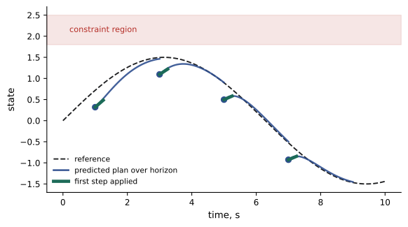
Model predictive control (MPC) solves an optimization at every control step: using a model, it plans the best sequence of controls over a short horizon (for example the next one or two seconds), subject to constraints on states and inputs, applies only the first control, then re-plans at the next step with fresh measurements. MPC handles constraints explicitly (torque limits, friction cones for feet, obstacle avoidance) and can anticipate future references. Its cost is computation: solving optimizations at 50 to 1,000 Hz requires efficient solvers and often simplified models. MPC is now standard in legged locomotion, autonomous driving and drone racing, and sampling-based variants such as MPPI work with arbitrary models, including learned ones.

Whole-body control for legged and humanoid robots

Legged robots and humanoids must coordinate dozens of joints while managing contacts with the ground and objects, keeping balance and respecting torque and friction limits. Whole-body controllers formulate this as an optimization at each control step (often a quadratic program): track several tasks, such as body height and orientation, swing foot trajectories and hand positions, with priorities or weights, subject to the robot's dynamics, contact constraints and actuator limits. Higher-level MPC plans contact forces and body motion over a horizon, and whole-body control turns them into joint torques. In recent years, reinforcement learning (Lesson 9) has produced remarkably robust locomotion policies for quadrupeds and humanoids, often outperforming hand-designed controllers on rough terrain, while model-based whole-body control remains common for manipulation and precise tasks. Many systems combine them.

Tuning in practice

Controller tuning on real robots follows a careful process: start with low gains and limits, test with the robot unloaded and in a safe position, increase gains step by step while watching for oscillation, check performance across the full range of motion and payloads, and record the final values with the conditions under which they were validated. Step responses, frequency responses and logs of tracking errors guide adjustments. Many robot vendors provide auto-tuning tools for joint controllers, but application-level controllers, such as force control for a specific task, are tuned by the integrator. Gains that work for one payload or speed may not work for another, so gain scheduling adjusts them across operating conditions.

Learning-based controllers are tuned differently, through reward design, training ranges and observation choices rather than gains, but the same principle applies: validate the behaviour across the full operating range before trusting it on the real robot.

Finally, controllers should degrade gracefully. When a sensor fails or a limit is reached, the controller should bring the robot to a safe, controlled stop rather than reacting unpredictably, and these fault responses deserve as much testing as normal operation.