Motion planning

Knowing where it is and what surrounds it, a robot must decide how to move: a path for a mobile robot through a warehouse full of shelves and people, or a collision-free trajectory for an arm reaching into a cluttered bin. Motion planning finds such motions while respecting obstacles, joint and velocity limits, and sometimes dynamics, comfort or energy. Planning problems range from simple 2D navigation, solvable by searching a grid, to high-dimensional problems such as a seven-joint arm or a humanoid, where exhaustive search is impossible and randomized or optimization-based methods are used. This lesson covers configuration space and collision checking, graph search with Dijkstra and A*, sampling-based planners such as PRM and RRT, trajectory optimization, time parameterization of paths, local planning and costmaps for mobile robots, planning around people, and the growing role of learning in planning.

Configuration space

Planning is easiest to think about in configuration space (C-space): the space of all robot configurations, with one dimension per degree of freedom. A mobile robot moving in a plane has a 3D C-space (x, y, heading); a seven-joint arm has a 7D C-space of joint angles. Obstacles in the workspace map to forbidden regions of C-space (C-obstacles), and planning becomes finding a path for a point through the free space between them. For a round mobile robot, C-obstacles are simply the workspace obstacles inflated by the robot's radius, which is why navigation costmaps inflate obstacles. For arms, C-obstacles have complex shapes that cannot be computed explicitly, so planners test individual configurations with a collision checker that computes forward kinematics and checks the robot's geometry against the environment using efficient libraries such as FCL.

Graph search

If the space is discretized, planning becomes graph search. Dijkstra's algorithm expands nodes in order of their cost from the start and finds the lowest-cost path. A* adds a heuristic estimate of the remaining cost to the goal, expanding nodes in order of f = g + h, where g is the cost so far and h is the heuristic. If the heuristic never overestimates the true remaining cost (it is admissible), A* still finds an optimal path but explores far fewer nodes, because it focuses the search toward the goal.

import heapq
import numpy as np
# Grid path planning: Dijkstra versus A* on a warehouse-like map
rng = np.random.default_rng(7)
h, w = 60, 80
grid = np.zeros((h, w), dtype=bool)
for c in range(10, 75, 10):                 # shelving rows with gaps
    grid[5:55, c:c + 3] = True
    gap = rng.integers(10, 45)
    grid[gap:gap + 4, c:c + 3] = False
grid[rng.random((h, w)) < 0.04] = True       # scattered clutter
start, goal = (30, 2), (30, 77)
grid[start] = grid[goal] = False

moves = [(1, 0, 1.0), (-1, 0, 1.0), (0, 1, 1.0), (0, -1, 1.0),
         (1, 1, 1.414), (1, -1, 1.414), (-1, 1, 1.414), (-1, -1, 1.414)]

def plan(use_heuristic):
    def heur(p):
        if not use_heuristic:
            return 0.0
        dy, dx = abs(p[0] - goal[0]), abs(p[1] - goal[1])
        return max(dy, dx) + 0.414 * min(dy, dx)     # octile distance, admissible
    frontier = [(heur(start), 0.0, start)]
    cost = {start: 0.0}
    expanded = 0
    while frontier:
        f, g, p = heapq.heappop(frontier)
        if g > cost[p]:
            continue
        expanded += 1
        if p == goal:
            return g, expanded
        for dy, dx, c in moves:
            q = (p[0] + dy, p[1] + dx)
            if 0 <= q[0] < h and 0 <= q[1] < w and not grid[q]:
                ng = g + c
                if ng < cost.get(q, 1e9):
                    cost[q] = ng
                    heapq.heappush(frontier, (ng + heur(q), ng, q))
    return None, expanded

for name, use in [("Dijkstra", False), ("A*", True)]:
    length, n = plan(use)
    print(f"{name:9s} path cost {length:6.2f} cells, nodes expanded {n:5d}")
print(f"free cells in map: {int((~grid).sum())}")

Dijkstra  path cost 102.39 cells, nodes expanded  3580
A*        path cost 102.39 cells, nodes expanded  1605
free cells in map: 3693

Both algorithms find the same optimal path, but Dijkstra expands almost every free cell in the map, while A*, guided by the octile distance heuristic suited to eight-connected grids, expands less than half as many. In larger maps the savings are greater. Variants are widely used in robotics: weighted A* trades optimality for speed, D* Lite and other incremental planners repair paths quickly when new obstacles appear, and hybrid A* plans for car-like robots that cannot turn in place by searching over motion primitives that respect turning radius. State lattice planners precompute feasible motion primitives and search over them.

Sampling-based planners

For high-dimensional C-spaces, discretizing every dimension is impossible: a 7D grid with 100 values per joint would have 10¹⁴ cells. Sampling-based planners instead sample random configurations, keep those that are collision-free, and connect them:

• Probabilistic roadmaps (PRM) build a graph of random free configurations connected by short collision-free edges, then search it. They suit multiple queries in a static environment.
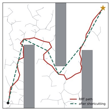
• Rapidly-exploring random trees (RRT) grow a tree from the start toward random samples, quickly exploring large spaces. RRT-Connect grows trees from start and goal and tries to join them, often finding paths in milliseconds.
• RRT* and related optimal planners continue refining to approach the shortest path as samples increase.

These planners are probabilistically complete: if a path exists, the probability of finding one approaches one as sampling continues. They struggle with narrow passages, where free space is a tiny fraction of the volume. The Open Motion Planning Library (OMPL), used through MoveIt 2, provides many such planners.

Trajectory optimization

Paths from sampling planners are often jagged and must be shortened and smoothed. Trajectory optimization instead treats the whole trajectory as variables and minimizes a cost (length, smoothness, effort, time) subject to constraints (no collisions, joint limits, dynamics). Methods such as CHOMP, STOMP and TrajOpt optimize trajectories for arms; direct collocation and multiple shooting handle dynamics for legged robots and drones. Optimization produces smooth, high-quality motions but can get stuck in local minima, for example on the wrong side of an obstacle, so it is often initialized from a sampling-based plan. Model predictive control (Lesson 8) applies the same idea repeatedly over a short horizon.

Time parameterization

A geometric path says where to go, not how fast. Time parameterization assigns timing so the robot respects velocity, acceleration and sometimes jerk limits. The simplest profile for a single joint is trapezoidal: accelerate at the maximum rate, cruise at maximum velocity, then decelerate. If the move is too short to reach cruise speed, the profile becomes triangular. Multi-joint paths are parameterized so all joints stay within limits simultaneously, using algorithms such as time-optimal path parameterization (TOPP) or iterative methods in MoveIt.

Local planning and costmaps for mobile robots

Mobile robots usually split navigation into a global planner, which finds a route across the map (for example A* or a lattice planner on a costmap), and a local planner or controller, which runs at 10 to 50 Hz, follows the route and avoids obstacles detected by sensors in real time. Costmaps combine layers: the static map, obstacles from current sensor data, inflation around obstacles that raises cost near walls and shelves, and special zones such as keep-out areas or speed limits. Local planners include the dynamic window approach (DWA), which samples feasible velocities and scores the resulting short trajectories; regulated pure pursuit, a geometric path follower; and model predictive path integral control (MPPI), which samples many trajectories in parallel and blends them by cost. The Nav2 stack in ROS 2 offers these as plugins, orchestrated by behaviour trees that also handle recovery behaviours such as backing up or clearing the costmap when the robot gets stuck.

Planning around people

Robots in hospitals, airports and offices share space with people, who move unpredictably and expect robots to behave politely. Social navigation goes beyond avoiding collisions: keeping comfortable distances, passing on the expected side, not cutting through groups, yielding at doorways, and moving in ways that make the robot's intentions legible. Planners use predictions of human motion, from constant-velocity models to learned trajectory predictors, and cost terms for social norms. Speed limits near people are also a safety requirement (Lesson 12).

Learning and planning

Learning increasingly assists planning. Learned heuristics and sampling distributions focus classical planners on promising regions; learned collision checkers speed up queries; and generative models, including diffusion models trained on many demonstrations, can propose whole trajectories that are then checked and refined. End-to-end learned navigation and manipulation policies (Lessons 9 to 11) implicitly plan, but in deployed systems they are usually combined with classical collision checking and safety constraints, since a planner's guarantees about obstacles are hard to obtain from a neural network alone.

Planning for manipulation

Manipulation planning has particular challenges. The robot must plan not only for the arm but also for the grasped object, which becomes part of the robot for collision checking. Approach and retreat motions must be planned so the gripper moves straight onto and away from the object. Placement requires choosing a stable pose for the object. Tasks involving several steps, such as clearing a table, combine task planning (which object to move first and where) with motion planning for each step, an area known as task and motion planning (TAMP). When objects are uncertain or partially hidden, planners may include actions that gather information, such as moving the camera to look behind an obstacle.

In practice, MoveIt 2 provides a widely used framework for arm motion planning in ROS 2, integrating IK solvers, planners from OMPL and others, collision checking, trajectory processing and execution. Learning-based grasp predictors and policies are often combined with MoveIt for the collision-free motions between grasps.

Planning time also matters in practice. A planner that takes several seconds per query may be acceptable for a robot loading a machine every few minutes, but not for a picking robot handling hundreds of items an hour. Engineers measure planning time distributions, set time budgets, cache plans for repeated motions, and fall back to simpler strategies when planning fails within the budget.

Whatever planner is used, plans should be validated before execution: checking for collisions with an up-to-date scene, verifying limits, and monitoring execution so the robot can stop and replan if the world changes.

Planners for mobile robots and arms are increasingly evaluated on standard benchmarks, but the real test is the deployed environment, where clutter, people and unexpected objects reveal gaps that benchmarks miss.