Localization, mapping and SLAM

A mobile robot needs to know where it is and what its surroundings look like: it needs a map, and it needs its position on that map. If a good map exists, the robot localizes against it. If no map exists, it must build one while keeping track of its own position on the map it is building, a chicken-and-egg problem called simultaneous localization and mapping (SLAM). SLAM was one of the central research problems of robotics for two decades and is now mature enough to run on robot vacuums, warehouse robots, phones and headsets, yet it still fails in long featureless corridors, changing environments and crowds. This lesson covers map representations, Monte Carlo localization with particle filters, occupancy grid mapping, the SLAM problem and its graph-based solution, loop closure and place recognition, lidar and visual SLAM systems, and the emerging use of semantic and learned maps.

Map representations

• Occupancy grids divide space into cells, each storing the probability that it is occupied. They are simple, work well with lidar, and support path planning directly. 2D grids are standard for indoor ground robots; 3D voxel grids and octrees (for example OctoMap) represent volumes.
• Feature or landmark maps store the positions of distinctive points, such as visual features or reflectors, and are compact.
• Point cloud and mesh maps store dense geometry, used for 3D localization and inspection.
• Topological maps represent places as nodes and connections as edges, useful for long-range route planning.
• Semantic maps add labels: rooms, doors, shelves, objects, supporting task-level commands such as "go to the kitchen".

Many systems use several layers: a metric map for local navigation, a topological graph for routes, and semantic labels for tasks.

Monte Carlo localization

Localization against a known map must handle multimodal uncertainty: in a building with repeated corridors, the robot may plausibly be in several places at once. Particle filters represent the belief as a set of samples (particles), each a hypothesized pose. Each cycle moves every particle according to the motion model with noise, weights it by how well the sensor reading matches what the map predicts at that pose, and resamples particles in proportion to their weights, so unlikely hypotheses die out and likely ones multiply. This is Monte Carlo localization (MCL), and the adaptive version (AMCL) is the standard localizer in the ROS 2 Nav2 stack.

import numpy as np
# Monte Carlo localization in a 1D corridor with doors
rng = np.random.default_rng(6)
length = 50.0
doors = np.array([5.0, 9.0, 24.0, 33.0, 36.0])     # door positions along the corridor, m
def near_door(x):
    return np.min(np.abs(x[:, None] - doors[None, :]), axis=1) < 0.75

n = 3000
particles = rng.uniform(0, length, n)              # global uncertainty: the robot could be anywhere
true_x = 2.0
for step in range(1, 31):
    true_x += 1.0
    particles = particles + 1.0 + rng.normal(0, 0.1, n)                   # motion update with noise
    sees_door = abs(true_x - doors).min() < 0.75
    z = sees_door if rng.random() < 0.95 else not sees_door                # door sensor right 95 % of the time
    w = np.where(near_door(particles) == z, 0.95, 0.05)                    # measurement likelihood
    w = np.where((particles < 0) | (particles > length), 0.0, w)           # outside the corridor is impossible
    w /= w.sum()
    particles = particles[rng.choice(n, n, p=w)]                           # resample
    if step in (1, 4, 8, 12, 20, 30):
        hist, edges = np.histogram(particles, bins=100, range=(0, length))
        mode = edges[hist.argmax()] + 0.25
        share = np.mean(np.abs(particles - true_x) < 1.0)
        print(f"step {step:2d}: true {true_x:5.1f} m, most likely {mode:5.1f} m, {share:4.0%} of particles within 1 m of the truth")

step  1: true   3.0 m, most likely  41.8 m,   4% of particles within 1 m of the truth
step  4: true   6.0 m, most likely  25.2 m,  12% of particles within 1 m of the truth
step  8: true  10.0 m, most likely  10.2 m,  65% of particles within 1 m of the truth
step 12: true  14.0 m, most likely  14.2 m,  79% of particles within 1 m of the truth
step 20: true  22.0 m, most likely  22.2 m,  96% of particles within 1 m of the truth
step 30: true  32.0 m, most likely  31.8 m, 100% of particles within 1 m of the truth

At the start, the robot could be anywhere, and after the first few steps the most likely position is wrong because several places in the corridor look similar. As the robot moves past distinctive patterns of doors and walls, inconsistent hypotheses die out: by step 8 most particles cluster at the true position, and by step 30 all of them do. The robot never sees its position directly; it infers it from how sequences of observations match the map. In practice, AMCL uses lidar scans compared with an occupancy grid, adapts the number of particles to the uncertainty, and injects random particles to recover from failures such as being moved while switched off (the kidnapped robot problem).

Occupancy grid mapping

When the robot's poses are known, building an occupancy grid from range sensors is straightforward. For each scan, cells along each beam up to the hit point are evidence of free space, and the cell at the hit point is evidence of an obstacle. Each cell's probability is updated with Bayes' rule, conveniently in log-odds form, l = log(p / (1 − p)), where each observation adds a fixed increment:

Log-odds updates are additions, so they are fast and numerically stable, and clamping the values lets the map adapt when furniture moves.

The SLAM problem

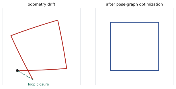
In SLAM, neither the map nor the poses are known. Errors in pose estimation corrupt the map, and errors in the map corrupt localization, so drift accumulates: after driving around a large loop, a robot using only odometry and scan matching will find that its start and end positions do not line up. Early solutions used EKF-SLAM, estimating robot pose and landmark positions jointly in one large filter, and FastSLAM, combining particles for the trajectory with small filters for landmarks (the basis of the widely used GMapping). Modern systems use graph-based SLAM:

• Front end: processes sensor data to produce constraints between poses, using scan matching or visual odometry between consecutive frames, and loop closure detection when the robot revisits a place.
• Back end: builds a pose graph, with nodes for robot poses and edges for constraints with their uncertainties, and solves a nonlinear least-squares optimization for the poses that best satisfy all constraints (Lesson 5).

When a loop closure is added, the optimizer distributes the accumulated error around the loop, snapping the map into consistency.

Loop closure and place recognition

Detecting that the robot has returned to a previously visited place is the key to bounded error, and also a major source of failure: a false loop closure (wrongly believing two different places are the same) can catastrophically distort the map. Place recognition methods include bag-of-visual-words matching of image features, global descriptors of lidar scans (such as Scan Context), and learned descriptors from neural networks that are robust to lighting and viewpoint changes. Candidate closures are verified geometrically, by aligning scans or matching features in 3D, and back ends use robust cost functions that can reject inconsistent closures.

Lidar and visual SLAM systems

• 2D lidar SLAM: slam_toolbox (the default in ROS 2 Nav2) and Cartographer build occupancy grids with pose-graph optimization, used on most indoor service and warehouse robots.
• 3D lidar SLAM and odometry: methods such as LOAM and its descendants, and lidar-inertial odometry (for example FAST-LIO and LIO-SAM), which tightly fuse IMU data for accurate motion estimation outdoors and on fast platforms.
• Visual SLAM: feature-based systems such as ORB-SLAM3 track features across frames, supporting monocular, stereo and RGB-D cameras, and visual-inertial variants (for example VINS-Mono and OpenVINS) fuse IMU data. Monocular systems cannot observe absolute scale without an IMU or known object sizes.
• Dense and learned methods: dense RGB-D reconstruction, and neural representations such as neural radiance fields and 3D Gaussian splatting, which produce photorealistic maps and are increasingly integrated with SLAM.

Choosing among them depends on the environment (indoor, outdoor, lighting), the sensors available, compute limits and the required accuracy.

Semantic and changing maps

Robots that take instructions in language need maps with meaning. Semantic SLAM attaches object detections and labels to map elements, and recent systems build open-vocabulary 3D scene graphs using vision-language features, so a robot can find "the charging cable near the blue chair". Real environments also change: furniture moves, doors open and close, shelves fill and empty. Long-term mapping systems distinguish static structure from movable objects, update maps over time, and localize robustly despite changes. Crowds of people, which occlude sensors and move constantly, remain a challenge for both localization and mapping in busy public spaces.

Localization in practice

Deployed mobile robots usually build their map once, during a supervised mapping run, and then localize against it during daily operation, updating the map when the environment changes significantly. Operators annotate the map with zones, docking stations, speed limits and named locations. Good practice includes mapping when the space is in its typical state, adding reflective markers or other features to long featureless corridors, monitoring localization confidence and stopping the robot safely if it becomes lost, and planning procedures for relocalization after maintenance.

Outdoors, GNSS provides absolute position, but near tall buildings, under trees and indoors it degrades or disappears, so outdoor robots combine it with lidar or visual localization and odometry. Agricultural robots often use RTK GNSS for centimetre accuracy in open fields, switching to other methods under canopies.

Indoor robots that move between floors add further challenges: elevators interrupt sensing and odometry, and each floor needs its own map. Fleet systems therefore integrate with building elevators and doors and keep multi-floor maps with explicit transitions.

Finally, mapping and localization performance should be measured, not assumed. Teams record ground-truth trajectories with motion capture or survey markers in test areas, compare them with the robot's estimates, and track localization failures per kilometre driven as a key reliability metric for deployed fleets.