Generative models for images and video

The models in earlier lessons analyse images: they classify, detect, segment and describe. Generative models do the reverse, producing new images, editing existing ones, filling in missing regions, increasing resolution and, increasingly, generating video. Since about 2021, diffusion models have made it possible to generate photorealistic images from text descriptions, transforming design, advertising, entertainment and visual effects, and raising serious concerns about deepfakes, consent and copyright. This lesson explains the main families of generative image models, autoencoders, generative adversarial networks and diffusion models, how text conditions them, how they are evaluated, how they are used, including to create training data for other vision models, and the risks and safeguards that accompany them.

Modelling the distribution of images

A generative model learns the probability distribution of its training images, \(p(\mathbf{x})\), so that it can draw new samples that look as if they came from the same distribution. Images are extremely high-dimensional (a 512 × 512 colour image has 786,432 values), but natural images occupy a tiny, structured part of that space, which is what makes learning possible. Generative models also learn conditional distributions, such as \(p(\mathbf{x} \mid \text{text})\) for text-to-image generation, or \(p(\text{full image} \mid \text{masked image})\) for inpainting.

Autoencoders and variational autoencoders

An autoencoder has an encoder that compresses an image into a small latent vector and a decoder that reconstructs the image from it, trained to minimize reconstruction error. Autoencoders learn compact representations but are not good generators, because their latent spaces have gaps: decoding a random latent vector gives nonsense. A variational autoencoder (VAE, 2013) makes the encoder output a distribution over latents and adds a penalty, the KL divergence from a standard normal distribution, that keeps the latent space smooth and filled, so that decoding a random normal vector gives a plausible image. VAEs train stably but their images tend to be blurry, because the reconstruction loss averages over plausible details. Today their main role is as the compression stage of latent diffusion models: an autoencoder maps images to a latent space perhaps 8 times smaller in each spatial dimension, where generation is far cheaper.

Generative adversarial networks

A generative adversarial network (GAN, 2014) trains two networks against each other. The generator turns random noise into images; the discriminator tries to tell generated images from real ones. The generator is trained to fool the discriminator, and as both improve, generated images become more realistic. The minimax objective is

GANs produce sharp images and generate them in a single network pass, so they are fast. StyleGAN (2018 to 2021) generated faces indistinguishable from photographs to most viewers, and GANs remain in use for super-resolution, image-to-image translation (for example turning sketches or semantic maps into photographs) and real-time applications. But GAN training is notoriously unstable, sensitive to architecture and hyperparameters, and prone to mode collapse, in which the generator produces only a few kinds of output that fool the discriminator rather than the full variety of the data. These problems limited GANs' ability to model very diverse datasets such as all the images on the web.

Diffusion models

Diffusion models (2015, made practical in 2020) take a different approach. A fixed forward process gradually destroys an image by adding Gaussian noise over many steps until it is pure noise; a neural network is trained to reverse the process one step at a time, removing a little noise at each step. After \(t\) steps, a noisy image can be written directly as

where \(\bar\alpha_t\) falls from 1 to near 0 according to a noise schedule. The network \(\boldsymbol{\epsilon}_\theta(\mathbf{x}_t, t)\) is trained with a simple objective: given a noisy image and the step, predict the noise that was added,

Predicting the noise is equivalent to estimating the score, the gradient of the log density of noisy images, which points toward more probable images. To generate, the model starts from pure noise and applies the learned denoising step repeatedly.

import numpy as np

# A one-dimensional diffusion model: data is a mixture of two narrow Gaussians at -2 and +2.
# The forward process adds noise; the reverse process uses the exact score of the noisy data to denoise.
rng = np.random.default_rng(0)
T = 200
betas = np.linspace(1e-4, 0.05, T)
alphas = 1 - betas
abar = np.cumprod(alphas)
for t in (0, 20, 50, 100, 199):
    snr = abar[t] / (1 - abar[t])
    print(f"step {t + 1:3d}: signal scale {np.sqrt(abar[t]):.3f}, noise scale {np.sqrt(1 - abar[t]):.3f}, SNR {snr:9.3f}")

mus, s0 = np.array([-2.0, 2.0]), 0.3
def score(x, t):                              # gradient of log density of the noisy data at step t
    m = np.sqrt(abar[t]) * mus[None, :]
    v = abar[t] * s0 ** 2 + (1 - abar[t])
    logw = -(x[:, None] - m) ** 2 / (2 * v)
    w = np.exp(logw - logw.max(axis=1, keepdims=True)); w /= w.sum(axis=1, keepdims=True)
    return (w * (m - x[:, None]) / v).sum(axis=1)

x = rng.normal(0, 1, 20000)                   # start from pure noise
for t in range(T - 1, -1, -1):                # DDPM reverse steps using eps = -sqrt(1 - abar) * score
    eps = -np.sqrt(1 - abar[t]) * score(x, t)
    x = (x - betas[t] / np.sqrt(1 - abar[t]) * eps) / np.sqrt(alphas[t])
    if t > 0:
        x += np.sqrt(betas[t]) * rng.normal(size=x.shape)
print(f"generated samples: {np.mean(x < 0):.1%} near -2 and {np.mean(x > 0):.1%} near +2; means {x[x < 0].mean():+.2f} and {x[x > 0].mean():+.2f}; spread {x[x > 0].std():.2f} (data 0.30)")

step   1: signal scale 1.000, noise scale 0.010, SNR  9999.000
step  21: signal scale 0.973, noise scale 0.231, SNR    17.735
step  51: signal scale 0.850, noise scale 0.528, SNR     2.593
step 101: signal scale 0.525, noise scale 0.851, SNR     0.381
step 200: signal scale 0.078, noise scale 0.997, SNR     0.006
generated samples: 50.3% near -2 and 49.7% near +2; means -2.00 and +1.99; spread 0.31 (data 0.30)

In this toy, the "data" consists of values clustered around −2 and +2. The forward process reduces the signal-to-noise ratio from very high to nearly zero over 200 steps. Starting from pure noise, the reverse process, guided by the score, recovers both modes in the right proportions with the right spread, with no mode collapse. Real image diffusion models do the same in hundreds of thousands of dimensions, with a U-Net or transformer learning the score from data instead of computing it exactly.

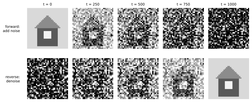
Diffusion models train stably, cover the full diversity of the data and produce excellent quality, but sampling is slow because it needs many network evaluations. Faster samplers (DDIM and ODE solvers) reduce the steps from about 1,000 to 20 to 50, and distillation methods (consistency models, adversarial distillation) produce good images in one to four steps.

Latent diffusion and text conditioning

Running diffusion on full-resolution pixels is expensive. Latent diffusion (2022), the basis of Stable Diffusion, first compresses images with a VAE into a smaller latent space and runs diffusion there, reducing compute by an order of magnitude or more. Text conditioning works by encoding the prompt with a text encoder (from CLIP or a language model, Lesson 7) and injecting the text embeddings into the denoising network through cross-attention layers, so each denoising step is guided by the prompt. The denoising networks have evolved from convolutional U-Nets to diffusion transformers (DiT), which scale better with compute, and to flow-matching models that learn straighter paths from noise to data.

Classifier-free guidance strengthens the influence of the prompt. During training, the text condition is randomly dropped, so the same network learns both conditional and unconditional predictions; at sampling, the prediction is extrapolated away from the unconditional one:

with guidance scale \(w\) typically 3 to 10. Higher guidance gives images that follow the prompt more closely but are less diverse and can look oversaturated.

Editing, control and video

Diffusion models do much more than generate from scratch:

• Inpainting and outpainting fill masked regions or extend an image beyond its borders, consistent with the surrounding content.
• Image-to-image translation starts the reverse process from a partially noised version of an input image, preserving its layout while changing style or content.
• Control signals such as edge maps, depth maps, human poses or segmentation maps (for example ControlNet) let users fix the composition precisely while the model fills in appearance.
• Personalization methods (DreamBooth, LoRA fine-tuning) teach a model a specific person, product or style from a handful of images.
• Super-resolution models increase image resolution, and diffusion-based restoration removes noise, blur and compression artifacts.
• Video diffusion models generate short clips by modelling time as an extra dimension, using spatio-temporal attention in a compressed latent space; keeping objects, physics and identity consistent over many seconds remains a frontier.

Evaluating generative models

Evaluating generated images is difficult, because there is no single correct output. Common measures:

• Fréchet Inception Distance (FID) compares the statistics of features of real and generated images, extracted by a pretrained network (originally Inception-v3). Modelling each feature set as a Gaussian with mean \(\boldsymbol\mu\) and covariance \(\Sigma\):

import numpy as np
from scipy.linalg import sqrtm

# Frechet Inception Distance (FID) between feature distributions, here with 64-dimensional synthetic features
rng = np.random.default_rng(0)
d, n = 64, 5000
A = rng.normal(0, 1, (d, d)) / np.sqrt(d)
real = rng.normal(0, 1, (n, d)) @ A + 1.0

def fid(x, y):
    m1, m2 = x.mean(0), y.mean(0)
    c1, c2 = np.cov(x, rowvar=False), np.cov(y, rowvar=False)
    cs = sqrtm(c1 @ c2).real
    return float(((m1 - m2) ** 2).sum() + np.trace(c1 + c2 - 2 * cs))

cases = {
    "second sample of real data": rng.normal(0, 1, (n, d)) @ A + 1.0,
    "generator with slight mean shift": rng.normal(0, 1, (n, d)) @ A + 1.1,
    "generator with low diversity (mode collapse)": 0.5 * (rng.normal(0, 1, (n, d)) @ A) + 1.0,
    "generator with wrong structure": rng.normal(0, 1, (n, d)) * 0.45 + 1.0,
}
for name, fake in cases.items():
    print(f"{name:45s} FID {fid(real, fake):6.2f}")

second sample of real data                    FID   0.30
generator with slight mean shift              FID   0.99
generator with low diversity (mode collapse)  FID  16.37
generator with wrong structure                FID  28.35

FID is low for samples from the same distribution and rises both for shifted means and for reduced diversity, which is how it detects mode collapse that a quality-only measure would miss. FID has limitations: it depends on the feature network, which was trained on ImageNet and may not capture what matters for faces or art; it needs many samples (at least 10,000 for stable values); and it does not measure whether images follow their prompts.

• CLIP score measures the similarity between a generated image and its prompt in CLIP's embedding space (Lesson 7), estimating prompt adherence.
• Precision and recall for generative models separate fidelity (are samples realistic?) from coverage (do they cover the variety of real images?).
• Human evaluation, typically pairwise preference between models on a set of prompts, remains the most trusted measure of overall quality, and benchmark arenas rank models by thousands of human votes.

Synthetic data for vision

Generated and rendered images are increasingly used to train other vision models, especially where real data is scarce, expensive, private or dangerous to collect: rare defects, unusual road situations for autonomous driving, medical conditions, or robots learning to grasp. Sources include physics-based rendering from 3D models and game engines (which give perfect labels for free, including depth and segmentation), and generative models conditioned on labels or layouts. The main challenge is the domain gap: models trained on synthetic data can learn its artifacts and fail on real images. Domain randomization (varying textures, lighting and backgrounds widely so that reality looks like just another variation), mixing synthetic with real data, and evaluating on real held-out data mitigate this.

Risks and safeguards

Image generation creates serious risks. Deepfakes, realistic images and videos of real people doing or saying things they never did, are used for fraud, harassment, non-consensual intimate imagery and political disinformation. Generated images can reproduce copyrighted works and artistic styles from their training data, raising unresolved legal questions about training on copyrighted images that are the subject of lawsuits in several countries. Models also reproduce and amplify biases in their training data, for example in whom they depict for prompts about professions. Safeguards include:

• Filtering training data and prompts, and refusing to generate certain content, such as sexual images of real people or of minors.
• Watermarking generated images, and attaching content credentials (C2PA) that record how an image was created.
• Detection tools that classify images as generated, though these are imperfect and can be evaded.
• Laws and policies: several Canadian provinces and many US states have laws against non-consensual intimate images that cover altered or synthetic images, and election laws increasingly address deceptive synthetic media. Platform policies require labelling of AI-generated content.

For practitioners, responsible use includes disclosing AI-generated content where viewers could be misled, obtaining consent before generating images of real people, respecting licences and artists' rights, and evaluating outputs for bias.