
AI-350 · Lesson 2 of 12 · 28 min
Image processing, features and geometric transforms
Lesson 1 showed how images are formed and how convolution with small kernels smooths an image or finds its edges. This lesson builds the rest of the classical image processing toolkit that still underpins much practical computer vision: adjusting brightness and contrast, choosing colour spaces, thresholding and morphology for segmentation in controlled settings, detecting edges, lines and corners, describing and matching local features between images, and the geometric transformations, including the homography, that relate views of the world. The lesson ends with RANSAC, a remarkably general method for fitting models to data contaminated by outliers. Deep networks now handle most recognition tasks, but these methods remain the basis of document scanning, panorama stitching, industrial inspection, augmented reality and the geometric stages of 3D reconstruction (Lessons 9 and 10), and they are fast, explainable and need no training data.
Point operations and histograms
Point operations change each pixel independently of its neighbours, according to a mapping from input to output intensity. The image histogram, the count of pixels at each intensity, shows how the intensities are distributed and guides these mappings:
- Brightness and contrast: \(g = a f + b\), where \(a > 1\) increases contrast and \(b\) shifts brightness; values are clipped to the valid range.
- Gamma correction: \(g = f^{\gamma}\) for intensities scaled to [0, 1], used to convert between linear sensor values and perceptually encoded image values (Lesson 1), and to brighten (γ < 1) or darken (γ > 1) mid-tones.
- Histogram equalization: maps intensities through the cumulative histogram so that the output uses the full range with roughly equal counts, revealing detail in low-contrast images. Adaptive versions such as CLAHE (contrast limited adaptive histogram equalization) equalize small tiles separately, which works well for medical images and scenes with uneven lighting.
Normalizing intensities, for example subtracting the mean and dividing by the standard deviation per channel, is also the first step of almost every neural network input pipeline.
Colour spaces
RGB is how cameras and displays work, but other colour spaces separate properties that matter for analysis:
- HSV (hue, saturation, value) separates the colour (hue) from its brightness, so a simple threshold on hue can segment, say, ripe red fruit or a green screen in varying lighting.
- YCbCr separates luminance (Y) from two colour difference channels, the basis of JPEG and video compression, which store colour at lower resolution because human vision is less sensitive to colour detail.
- CIE L*a*b* is designed to be perceptually uniform, so that Euclidean distances roughly match perceived colour differences; it is used for colour measurement and quality control.
For neural networks, RGB input is standard and the network learns whatever colour transformations it needs; for classical pipelines, choosing the right colour space can turn a hard segmentation problem into a simple threshold.
Thresholding and morphology
In controlled settings, such as a conveyor with a uniform background or a scanned document, segmenting objects from the background can be as simple as a threshold: pixels brighter than \(T\) are foreground. Otsu's method chooses \(T\) automatically by maximizing the separation (between-class variance) of the two resulting groups of pixels in the histogram. Adaptive thresholding computes a local threshold for each region, handling uneven illumination in documents.
Binary masks from thresholding are cleaned up with morphological operations, which use a small structuring element (for example a 3 × 3 square or a disc):
- Erosion shrinks foreground regions, removing small specks and thin connections.
- Dilation grows them, filling small holes and gaps.
- Opening (erosion then dilation) removes small noise while preserving the size of larger objects; closing (dilation then erosion) fills small holes and joins nearby fragments.
Connected component labelling then assigns a label to each separate blob, from which properties such as area, centroid, bounding box and orientation are measured. A classical inspection system might threshold an image of parts on a backlit table, clean the mask with opening, label the components, and reject any part whose area or shape falls outside tolerance, all in a few milliseconds with no training data.
Edges and lines
The Sobel filters of Lesson 1 give the gradient at each pixel, but turning gradients into clean edges requires more steps. The Canny edge detector (1986), still widely used, works in four stages: smooth with a Gaussian to reduce noise; compute gradient magnitude and direction; thin edges to one pixel by non-maximum suppression along the gradient direction; and link edges with hysteresis thresholding, keeping weak edge pixels only if they connect to strong ones. Its two thresholds and the smoothing scale trade sensitivity against noise.
Straight lines and circles are found with the Hough transform. Each edge pixel votes for all the lines that could pass through it, parameterized by angle \(\theta\) and distance \(\rho\) from the origin, \(\rho = x\cos\theta + y\sin\theta\); lines supported by many edge pixels appear as peaks in the accumulator array of votes. The Hough transform is robust to gaps and clutter because a line needs only enough votes, not a continuous chain of pixels, and it is used for lane markings, document borders, and circular parts and pupils (with a circle parameterization).
Corners and keypoints
Edges are ambiguous for matching: a point on a straight edge can slide along the edge without changing its appearance (the aperture problem, Lesson 9). Corners, where the intensity changes in two directions, can be located precisely, so they make good keypoints for matching between images. The Harris detector examines the structure tensor, the matrix of summed gradient products in a small window,
whose eigenvalues are both large at a corner, one large and one small on an edge, and both small in a flat region. The response \(R\), with \(k\) about 0.04 to 0.06, is large and positive at corners, negative on edges and near zero in flat regions.
import numpy as np

# Harris corner detector on a synthetic image: a bright rectangle (four corners) and a long straight edge (no corners)
img = np.zeros((40, 40))
img[8:24, 6:20] = 1.0
img[:, 30:] = 0.6
rng = np.random.default_rng(0)
img += rng.normal(0, 0.02, img.shape)

def conv(x, k):
    kh, kw = k.shape
    p = np.pad(x, ((kh // 2,), (kw // 2,)), mode="edge")
    out = np.zeros_like(x)
    for i in range(kh):
        for j in range(kw):
            out += k[i, j] * p[i:i + x.shape[0], j:j + x.shape[1]]
    return out

sob = np.array([[-1, 0, 1], [-2, 0, 2], [-1, 0, 1]]) / 8
Ix, Iy = conv(img, sob), conv(img, sob.T)
g = np.outer([1, 4, 6, 4, 1], [1, 4, 6, 4, 1]) / 256.0  # Gaussian window
Sxx, Syy, Sxy = conv(Ix * Ix, g), conv(Iy * Iy, g), conv(Ix * Iy, g)
R = Sxx * Syy - Sxy ** 2 - 0.05 * (Sxx + Syy) ** 2      # Harris response
# non-maximum suppression in 7 x 7 neighbourhoods, keep strong responses
corners = []
for i in range(3, 37):
    for j in range(3, 37):
        if R[i, j] > 0.1 * R.max() and R[i, j] == R[i - 3:i + 4, j - 3:j + 4].max():
            corners.append((i, j, R[i, j]))
for i, j, r in sorted(corners, key=lambda c: -c[2]):
    print(f"corner at row {i:2d}, col {j:2d}  (response {r / R.max():.2f})")
print(f"response on the straight edge at (20, 30): {R[20, 30] / R.max():+.3f}; in a flat region at (32, 12): {R[32, 12] / R.max():+.3f}")corner at row 8, col 19 (response 1.00) corner at row 23, col 19 (response 0.98) corner at row 8, col 6 (response 0.96) corner at row 23, col 6 (response 0.96) response on the straight edge at (20, 30): -0.034; in a flat region at (32, 12): +0.000
The detector finds the four corners of the rectangle and gives a negative response on the long straight edge and zero in flat areas, exactly as the eigenvalue analysis predicts. Real images contain hundreds or thousands of such keypoints. Scale-invariant detectors such as the one in SIFT find keypoints as extrema of the difference of Gaussians across scale, so the same physical corner is detected whether it appears large or small.
Descriptors and matching
To match keypoints between images, each is given a descriptor, a vector summarizing the image patch around it in a way that is robust to changes in viewpoint, lighting and scale. SIFT (scale-invariant feature transform, 2004) divides the patch, rotated to its dominant gradient orientation, into a 4 × 4 grid and records an 8-bin histogram of gradient orientations in each cell, giving a 128-dimensional vector. ORB and other binary descriptors compare pairs of pixel intensities to produce compact bit strings that are very fast to match with Hamming distance, suiting real-time applications on phones and robots. Learned descriptors from neural networks (for example SuperPoint with SuperGlue or LightGlue matching) now outperform hand-designed ones in difficult conditions.
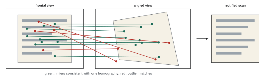
Matching compares each descriptor with those in the other image and takes the nearest neighbour. Many such matches are wrong, so filters are applied: Lowe's ratio test keeps a match only if the nearest neighbour is clearly closer than the second nearest (for example, a distance ratio below 0.8), and cross-checking keeps only matches that are mutual nearest neighbours. Even after filtering, a substantial fraction of matches are typically outliers, which is why robust estimation is essential.
Geometric transformations
Points in two images of the same scene are related by geometric transformations of increasing generality, written conveniently in homogeneous coordinates (Lesson 1), where a 2D point \((x, y)\) becomes \((x, y, 1)\):
| Transformation | Degrees of freedom | Preserves | Example |
|---|---|---|---|
| Translation | 2 | orientation, lengths, angles | shifting an image |
| Euclidean (rigid) | 3 | lengths and angles | rotating a scanned page |
| Similarity | 4 | angles and length ratios | zooming and rotating |
| Affine | 6 | parallel lines, area ratios | view of a distant plane, shear |
| Projective (homography) | 8 | straight lines | view of a plane from any angle; camera rotation |
A homography is a 3 × 3 matrix \(H\), defined up to scale, mapping points on one plane to another: \(\mathbf{x}' \sim H\mathbf{x}\). It describes two important situations exactly: views of a planar surface (a document, a facade, a floor) from different positions, and any two images taken by a camera rotating about its centre (the basis of panoramas). Each point match gives two linear equations in the entries of \(H\), so four matches determine it; with more matches, the direct linear transform (DLT) solves a least-squares problem using the singular value decomposition.
Applying a homography to warp an image, for example to produce a flat, rectangular "scan" of a document photographed at an angle, requires resampling: for each output pixel, compute where it comes from in the input image and interpolate (bilinear interpolation is the usual choice) between neighbouring input pixels.
Robust fitting with RANSAC
Least squares fits a model to all the data, and a few gross outliers can ruin it. RANSAC (random sample consensus, 1981) repeatedly fits the model to a minimal random sample (four matches for a homography, two points for a line), counts how many of all the data points agree with it within a tolerance (the inliers), and keeps the model with the most inliers, which is finally refitted to all its inliers.
import numpy as np

# Estimate a homography between two views of a planar document from noisy matches with outliers, using RANSAC
rng = np.random.default_rng(1)
H_true = np.array([[0.9, 0.12, 30.0], [-0.08, 1.05, 12.0], [0.0004, 0.0002, 1.0]])
def apply(H, p):
    q = np.c_[p, np.ones(len(p))] @ H.T
    return q[:, :2] / q[:, 2:]

n = 120
src = rng.uniform(0, 400, (n, 2))
dst = apply(H_true, src) + rng.normal(0, 1.0, (n, 2))       # 1-pixel noise
out = rng.choice(n, 45, replace=False)                        # 45 wrong matches (37%)
dst[out] = rng.uniform(0, 450, (45, 2))

def dlt(a, b):                                                # direct linear transform from 4 or more matches
    A = []
    for (x, y), (u, v) in zip(a, b):
        A.append([-x, -y, -1, 0, 0, 0, u * x, u * y, u])
        A.append([0, 0, 0, -x, -y, -1, v * x, v * y, v])
    _, _, Vt = np.linalg.svd(np.array(A))
    H = Vt[-1].reshape(3, 3)
    return H / H[2, 2]

def err(H):
    return np.linalg.norm(apply(H, src) - dst, axis=1)

H_all = dlt(src, dst)
print(f"least squares on all matches: median error {np.median(err(H_all)):6.1f} px")
best, best_in = None, 0
for it in range(500):
    idx = rng.choice(n, 4, replace=False)
    H = dlt(src[idx], dst[idx])
    inl = err(H) < 3.0
    if inl.sum() > best_in:
        best, best_in = inl, inl.sum()
H_r = dlt(src[best], dst[best])                              # refit on all inliers
true_inl = np.ones(n, bool); true_inl[out] = False
print(f"RANSAC: {best_in} inliers found ({(best & true_inl).sum()} true inliers of {true_inl.sum()}), median inlier error {np.median(err(H_r)[best]):.2f} px")
w = 1 - 45 / n
print(f"iterations needed for 99% confidence with {w:.0%} inliers and 4-point samples: {np.log(0.01) / np.log(1 - w ** 4):.0f}")least squares on all matches: median error 163.8 px RANSAC: 74 inliers found (74 true inliers of 75), median inlier error 1.12 px iterations needed for 99% confidence with 62% inliers and 4-point samples: 28
Least squares on all matches is useless here, with a median error of over 160 pixels, because the 37% outliers drag the solution far from the truth. RANSAC finds essentially all the true inliers and recovers the homography to about one pixel, the level of the noise. The number of iterations needed to find at least one all-inlier sample with probability \(p\) is
where \(w\) is the inlier fraction and \(s\) the sample size. With 62% inliers and \(s = 4\), only 28 iterations give 99% confidence, but with 20% inliers it would take over 2,800, which is why good matching filters and small minimal samples matter. RANSAC and its many refinements are used throughout geometric vision: estimating homographies, fundamental and essential matrices (Lesson 10), camera poses, and planes in 3D point clouds.
Worked problem
Planning a document scanner app
A phone app must turn a photo of a receipt on a table into a flat, readable scan. Outline a classical pipeline and the role of each step.
Show solution
- Convert to greyscale and smooth; detect edges with Canny.
- Find the receipt outline: the largest four-sided contour, or four strong lines from the Hough transform, giving the four corners.
- Compute the homography from the four corners to a rectangle with the receipt's aspect ratio, and warp the image with bilinear interpolation.
- Apply adaptive thresholding or contrast enhancement to make the text crisp for OCR (Lesson 11).
Answer: Edges, contour or line detection, a four-point homography and adaptive thresholding produce a good scan in milliseconds on a phone without any training data. Modern apps add a small neural network to find the document corners when the background is cluttered, combining learned and classical stages.
Common mistakes
MistakeFitting geometric models by least squares to raw feature matches.
InsteadUse RANSAC or another robust estimator; matches contain many outliers.
MistakeUsing RGB thresholds for colour segmentation under changing light.
InsteadThreshold hue in HSV or use a perceptual space, or learn a classifier.
MistakeMatching keypoints without filtering.
InsteadApply the ratio test and cross-checking before robust fitting.
MistakeWarping images by forward mapping each input pixel.
InsteadUse inverse mapping with interpolation to avoid holes.
MistakeAssuming a homography relates any two views of a scene.
InsteadIt is exact only for planar scenes or a rotating camera; general scenes need epipolar geometry.
Summary and key terms
- Point operations, gamma and histogram equalization adjust intensities; normalization prepares network inputs.
- Colour spaces such as HSV, YCbCr and L*a*b* separate properties useful for analysis.
- Thresholding (Otsu, adaptive), morphology and connected components segment objects in controlled settings.
- Canny finds clean edges; the Hough transform finds lines and circles robustly.
- Harris and scale-space detectors find corners; SIFT, ORB and learned descriptors enable matching with ratio tests.
- Homographies relate views of planes and rotating cameras; the DLT estimates them from four or more matches.
- RANSAC fits models robustly despite many outliers; iterations grow rapidly as the inlier fraction falls.
- Histogram equalization
- Remapping intensities to spread them evenly over the range.
- Otsu's method
- Automatic threshold selection maximizing between-class variance.
- Morphological opening
- Erosion followed by dilation, removing small noise.
- Canny edge detector
- A multi-stage edge detector with non-maximum suppression and hysteresis.
- Hough transform
- A voting method for detecting parameterized shapes such as lines.
- Harris detector
- A corner detector based on the structure tensor.
- Descriptor
- A vector summarizing the appearance around a keypoint.
- Ratio test
- Keeping a match only if it is clearly better than the second best.
- Homography
- A projective transformation between planes, a 3 × 3 matrix up to scale.
- RANSAC
- Random sample consensus, a robust model-fitting method.
Practice problems
Work each problem on paper first, then reveal the answer to check.
What does gamma 0.5 do to mid-tones?
Show answer
Brightens them.
Why use HSV for colour segmentation?
Show answer
Hue is separated from brightness, so thresholds are more robust to lighting.
What does morphological closing do?
Show answer
Fills small holes and joins nearby fragments.
Name the four stages of Canny.
Show answer
Smoothing, gradients, non-maximum suppression, hysteresis.
In Harris, what are the eigenvalues of M on an edge?
Show answer
One large, one small.
How long is a SIFT descriptor?
Show answer
128 numbers.
How many point matches determine a homography?
Show answer
Four.
RANSAC iterations for 99% confidence, 50% inliers, 4-point samples?
Show answer
\(\log 0.01/\log(1 - 0.0625) \approx 72\).
When is a homography exact for two views?
Show answer
For a planar scene or a camera rotating about its centre.
Why inverse mapping for warping?
Show answer
Every output pixel gets a value; forward mapping leaves holes.
Lesson quiz · 5 questions
Score 60% or more to complete this lesson.
Create a free account to save your progress, take quizzes and earn a certificate.