
AI-350 · Lesson 5 of 12 · 28 min
Detection and segmentation
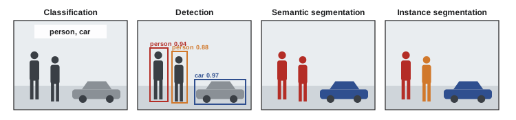
Classifying a whole image as "contains a dog" is rarely enough. A self-driving car must know where every pedestrian, vehicle and lane line is; a radiologist's tool must outline a tumour; a warehouse robot must find the exact shape of each parcel to grasp it. Object detection finds and labels each object with a bounding box; semantic segmentation labels every pixel with a class; instance segmentation separates individual objects pixel by pixel; and related tasks find keypoints such as human body joints. This lesson covers how these tasks are framed, the main model families, how they are evaluated, and the special issues raised by detecting and recognizing people.
The tasks
| Task | Output | Example use |
|---|---|---|
| Classification | One label (or several) per image | Photo tagging, defect present or not |
| Object detection | A box, class and confidence for each object | Vehicles and pedestrians for driver assistance |
| Semantic segmentation | A class for every pixel | Road, sidewalk and sky for navigation; land cover in satellite images |
| Instance segmentation | A mask for each individual object | Counting and measuring cells; robot grasping |
| Panoptic segmentation | Every pixel labelled with class and instance | Complete scene understanding |
| Keypoint detection | Coordinates of landmarks such as body joints | Pose estimation, sports analysis |
Bounding boxes and IoU
A detector outputs boxes, usually as corner coordinates \((x_1, y_1, x_2, y_2)\) or as centre, width and height. The standard measure of how well a predicted box matches a ground-truth box is intersection over union (IoU):
IoU is 1 for a perfect match and 0 for no overlap. A detection usually counts as correct if its IoU with an unmatched ground-truth box of the same class is at least 0.5, though stricter thresholds (up to 0.95) are used to reward precise localization.
Worked problem
IoU by hand
A ground-truth box spans (0, 0) to (10, 10) and a prediction spans (5, 0) to (15, 10). Compute IoU.
Show solution
- Intersection: x from 5 to 10, y from 0 to 10: area 50.
- Union: \(100 + 100 - 50 = 150\).
- IoU \(= 50/150 = 0.33\).
Answer: IoU is 0.33, below the usual 0.5 threshold, even though the prediction covers half the object. Shifting a box by half its width is a serious localization error, which IoU captures.
Detector families
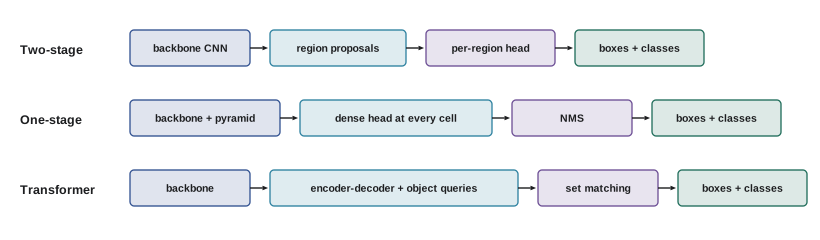
Detectors predict boxes at many candidate positions and keep the confident ones. Three generations of design are common:
- Two-stage detectors (R-CNN, Fast R-CNN, Faster R-CNN, 2014 to 2015): a region proposal network suggests a few thousand candidate boxes from the CNN feature map; a second stage classifies each and refines its coordinates. Accurate, and the basis of Mask R-CNN for instance segmentation.
- One-stage detectors (SSD, the YOLO family, RetinaNet): predict classes and box offsets directly at every location of one or more feature maps, often relative to preset anchor boxes of several shapes. Faster, and widely used for real-time detection on video and embedded devices. RetinaNet introduced focal loss, which down-weights the overwhelming number of easy background locations.
- Transformer-based detectors (DETR, 2020, and successors): treat detection as predicting a set of objects, using learned object queries and a matching loss, with no anchors or duplicate removal needed. Modern variants are both accurate and fast.
Most detectors use feature pyramids that combine coarse, semantically strong deep features with fine, high-resolution early features, so that both large and small objects are detected. Small objects remain the hardest case, since they occupy few pixels.
Non-maximum suppression
Dense detectors predict many overlapping boxes for the same object. Non-maximum suppression (NMS) removes duplicates: sort boxes by confidence, keep the highest, discard any remaining box whose IoU with it exceeds a threshold, and repeat.
import numpy as np

def iou(a, b):
    # boxes as (x1, y1, x2, y2)
    ix = max(0, min(a[2], b[2]) - max(a[0], b[0]))
    iy = max(0, min(a[3], b[3]) - max(a[1], b[1]))
    inter = ix * iy
    union = (a[2] - a[0]) * (a[3] - a[1]) + (b[2] - b[0]) * (b[3] - b[1]) - inter
    return inter / union

def nms(boxes, scores, thr=0.5):
    order = list(np.argsort(scores)[::-1])
    keep = []
    while order:
        i = order.pop(0)
        keep.append(int(i))
        order = [j for j in order if iou(boxes[i], boxes[j]) < thr]
    return keep

boxes = [(10, 10, 110, 210), (14, 18, 112, 214), (20, 5, 118, 200), (150, 40, 250, 220), (160, 50, 245, 230), (300, 300, 340, 330)]
scores = [0.92, 0.85, 0.60, 0.88, 0.75, 0.30]
print("IoU(box 0, box 1) =", round(iou(boxes[0], boxes[1]), 3))
print("IoU(box 0, box 3) =", round(iou(boxes[0], boxes[3]), 3))
for thr in (0.5, 0.8):
print(f"NMS at IoU threshold {thr}: keep boxes {nms(boxes, scores, thr)}")IoU(box 0, box 1) = 0.887 IoU(box 0, box 3) = 0.0 NMS at IoU threshold 0.5: keep boxes [0, 3, 5] NMS at IoU threshold 0.8: keep boxes [0, 3, 4, 2, 5]
With the common threshold of 0.5, NMS keeps one box per object (boxes 0, 3 and 5), discarding the near-duplicates around the first two objects. A looser threshold of 0.8 keeps duplicates whose overlap is below 0.8, such as box 4 (an offset second box on the car) and box 2. Too low a threshold, by contrast, merges genuinely separate objects that overlap, such as people in a crowd, which is one reason set-based transformer detectors that avoid NMS are attractive.
Evaluating detectors: precision, recall and AP
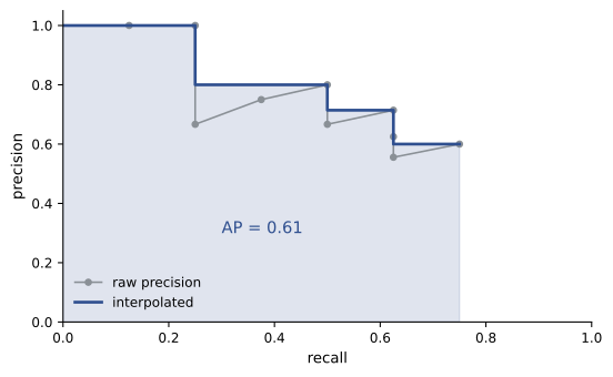
Each detection is a true positive if it matches an unmatched ground-truth object at the IoU threshold, or a false positive otherwise; unmatched ground-truth objects are false negatives. Ranking detections by confidence and moving the threshold down traces a precision-recall curve. Average precision (AP) is the area under it (with precision made non-increasing), summarizing performance across all thresholds:
Mean average precision (mAP) averages AP over classes. The COCO benchmark reports AP averaged over IoU thresholds from 0.5 to 0.95, written AP or AP@[.5:.95], as well as AP50 and AP75, and separately for small, medium and large objects.
import numpy as np

# detections for one class across a test set, sorted later by score; True = matched a ground truth at IoU >= 0.5
scores = np.array([0.95, 0.91, 0.88, 0.80, 0.77, 0.70, 0.62, 0.55, 0.43, 0.30])
correct = np.array([1, 1, 0, 1, 1, 0, 1, 0, 0, 1])
n_gt = 8                                   # objects of this class in the ground truth

order = np.argsort(-scores)
tp = np.cumsum(correct[order]); fp = np.cumsum(1 - correct[order])
precision = tp / (tp + fp); recall = tp / n_gt
for k in range(len(scores)):
    print(f"top {k + 1:2d} (score >= {scores[order][k]:.2f}): precision {precision[k]:.2f}, recall {recall[k]:.3f}")

# average precision: area under the precision-recall curve, with precision made non-increasing
p_interp = np.maximum.accumulate(precision[::-1])[::-1]
r = np.concatenate(([0.0], recall))
ap = np.sum((r[1:] - r[:-1]) * p_interp)
print(f"average precision (AP at IoU 0.5) = {ap:.3f}")top 1 (score >= 0.95): precision 1.00, recall 0.125 top 2 (score >= 0.91): precision 1.00, recall 0.250 top 3 (score >= 0.88): precision 0.67, recall 0.250 top 4 (score >= 0.80): precision 0.75, recall 0.375 top 5 (score >= 0.77): precision 0.80, recall 0.500 top 6 (score >= 0.70): precision 0.67, recall 0.500 top 7 (score >= 0.62): precision 0.71, recall 0.625 top 8 (score >= 0.55): precision 0.62, recall 0.625 top 9 (score >= 0.43): precision 0.56, recall 0.625 top 10 (score >= 0.30): precision 0.60, recall 0.750 average precision (AP at IoU 0.5) = 0.614
As the threshold falls, recall rises to 0.75 (6 of 8 objects found) while precision drifts down to 0.6. The area under the interpolated curve gives an AP of 0.61. Choosing an operating threshold is a separate, application-specific decision: a car's pedestrian detector needs very high recall, while a photo-tagging feature might prefer high precision.
Semantic and instance segmentation
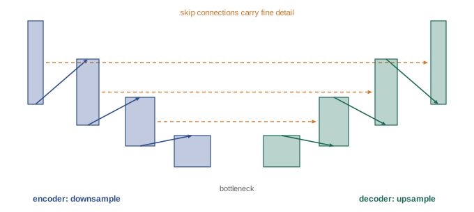
Segmentation networks must output a full-resolution map, but CNN backbones reduce resolution. Fully convolutional networks (FCN, 2015) replaced final fully connected layers with convolutions and upsampled the coarse output. U-Net (2015), developed for biomedical images, uses an encoder that downsamples and a decoder that upsamples, with skip connections passing fine detail from each encoder level to the matching decoder level; it remains a standard for medical and scientific segmentation, and the same shape underlies image diffusion models. DeepLab used dilated (atrous) convolutions to enlarge receptive fields without losing resolution. Instance segmentation adds a mask prediction to each detection, as in Mask R-CNN, or uses query-based transformer models such as Mask2Former that handle semantic, instance and panoptic segmentation in one architecture.
Since 2023, promptable foundation models such as Meta's Segment Anything (SAM) can segment almost any object given a click, box or text prompt, without task-specific training, and are now used to accelerate annotation and as components of larger systems.
Segmentation is evaluated per class with IoU (also called the Jaccard index) or the Dice coefficient \(2|A \cap B|/(|A| + |B|)\), averaged over classes as mean IoU. Pixel accuracy is easy to compute but dominated by large classes such as background.
import numpy as np

# 3 classes on a 10 x 10 image: 0 = background, 1 = road, 2 = pedestrian (small)
gt = np.zeros((10, 10), int); gt[6:, :] = 1; gt[2:6, 4:6] = 2
pred = gt.copy()
pred[6, :] = 0                      # misses the top row of road
pred[2:6, 4] = 0                    # misses half the pedestrian

def metrics(gt, pred, k):
    acc = (gt == pred).mean()
    ious, dices = [], []
    for c in range(k):
        inter = ((gt == c) & (pred == c)).sum()
        union = ((gt == c) | (pred == c)).sum()
        ious.append(inter / union)
        dices.append(2 * inter / ((gt == c).sum() + (pred == c).sum()))
    return acc, ious, dices

acc, ious, dices = metrics(gt, pred, 3)
print(f"pixel accuracy: {acc:.3f}")
for c, name in enumerate(("background", "road", "pedestrian")):
    print(f"{name:10s}: IoU {ious[c]:.3f}  Dice {dices[c]:.3f}  pixels in ground truth {(gt == c).sum()}")
print(f"mean IoU: {np.mean(ious):.3f}")pixel accuracy: 0.860 background: IoU 0.788 Dice 0.881 pixels in ground truth 52 road : IoU 0.750 Dice 0.857 pixels in ground truth 40 pedestrian: IoU 0.500 Dice 0.667 pixels in ground truth 8 mean IoU: 0.679
Pixel accuracy (86%) looks good, but the small pedestrian class, which matters most for safety, has IoU of only 0.5 because half its eight pixels were missed. Mean IoU (0.68) weights each class equally and exposes the problem. Safety-critical applications report per-class results and often weight errors on rare, important classes more heavily.
Annotation
Dense prediction tasks need costly labels: drawing a box takes about 7 to 30 seconds, and a precise polygon mask a minute or more per object, so a large segmentation dataset can cost millions of dollars to annotate. Annotation quality, consistency and clear guidelines (what counts as an object, how to handle occlusion) strongly affect model quality. Approaches to reduce cost include model-assisted labelling (a model proposes, a person corrects), promptable segmentation tools, active learning (labelling the examples the model is least sure about), weak supervision from image-level labels, and synthetic data rendered from 3D simulations with perfect labels.
Worked problem
Annotation budget
A dataset has 20,000 images with an average of 8 objects each. Boxes take 10 s per object, polygon masks 60 s, and model-assisted masks 20 s. At $12 per annotator-hour, compare the costs.
Show solution
- Objects: 160,000.
- Boxes: \(160{,}000 \times 10 = 1.6 \times 10^6\) s \(= 444\) h \(= \$5{,}300\).
- Masks: 2667 h \(= \$32{,}000\). Model-assisted masks: 889 h \(= \$10{,}700\).
Answer: About $5,300 for boxes, $32,000 for manual masks and $10,700 for model-assisted masks, before quality review, which typically adds 20 to 50%. Choosing the cheapest label type that meets the task's needs is a major design decision.
Detecting and recognizing people
Person detection, pose estimation and face analysis are among the most valuable and most sensitive vision applications. Face recognition compares an embedding of a face (Lesson 7) with stored embeddings to verify identity (one-to-one, as when unlocking a phone) or identify a person (one-to-many, searching a database). Accuracy has improved dramatically, but studies such as the US National Institute of Standards and Technology's evaluations have found error rates that vary with demographics for many algorithms, especially in less controlled images, and errors in one-to-many identification have led to wrongful arrests. Surveillance, tracking and biometric identification raise serious privacy and civil liberties concerns.
In Canada, biometric information such as facial templates is sensitive personal information under privacy law. In 2021 the federal Privacy Commissioner and provincial counterparts found that Clearview AI's scraping of billions of online images to build a facial recognition database violated Canadian privacy laws, and that the RCMP's use of it contravened the Privacy Act. Québec's Law 25 requires organizations to disclose the creation of biometric databases to the province's Commission d'accès à l'information in advance and generally to obtain express consent to verify identity with biometrics. Privacy commissioners have issued guidance on police use of facial recognition, and retailers using it have been found in breach of privacy law.
Responsible deployment involves evaluating accuracy across demographic groups and conditions, setting thresholds appropriate to the stakes, keeping humans responsible for consequential decisions, minimizing data collection and retention, and being transparent with the people affected.
Lesson 6 looks inside modern detectors: how positives are assigned, focal loss, DETR, panoptic segmentation and pose estimation.
Common mistakes
MistakeReporting AP without stating the IoU threshold.
InsteadSpecify AP50, AP75 or COCO AP@[.5:.95].
MistakeSetting the NMS threshold without considering crowded scenes.
InsteadTune it on validation data, or use set-based detectors.
MistakeJudging segmentation by pixel accuracy.
InsteadReport per-class IoU or Dice and mean IoU.
MistakeIgnoring small objects when choosing input resolution.
InsteadUse higher resolution, feature pyramids or tiling for small objects.
MistakeDeploying face recognition without demographic evaluation.
InsteadMeasure error rates across groups and conditions and keep humans in the loop.
Summary and key terms
- Detection outputs boxes, classes and confidences; segmentation labels pixels; instance segmentation separates objects.
- IoU measures box or mask overlap; 0.5 is the common match threshold.
- Two-stage, one-stage and transformer detectors trade accuracy and speed; feature pyramids help small objects.
- NMS removes duplicate detections by IoU.
- AP is the area under the precision-recall curve; mAP averages over classes and IoU thresholds.
- FCN, U-Net, DeepLab and Mask R-CNN segment images; promptable models segment almost anything.
- Mean IoU and Dice evaluate segmentation better than pixel accuracy.
- Biometric data is sensitive under Canadian privacy law; Law 25 regulates biometric databases.
- Bounding box
- A rectangle enclosing an object.
- Intersection over union
- Overlap area divided by union area of two regions.
- Anchor box
- A preset box shape relative to which a detector predicts offsets.
- Non-maximum suppression
- Removing overlapping lower-confidence detections.
- Average precision
- The area under the precision-recall curve.
- Semantic segmentation
- Labelling each pixel with a class.
- Instance segmentation
- Separating individual objects with masks.
- U-Net
- An encoder-decoder segmentation network with skip connections.
- Dice coefficient
- Twice the overlap divided by the sum of region sizes.
- Face verification
- Checking whether a face matches one claimed identity.
- Face identification
- Searching a database for the identity of a face.
Practice problems
Work each problem on paper first, then reveal the answer to check.
Boxes (0,0,4,4) and (2,2,6,6). IoU?
Show answer
Intersection 4; union 28; IoU = 0.143.
Why is IoU preferred over the distance between box centres?
Show answer
It accounts for size and shape and is scale-invariant.
What is the main speed difference between one-stage and two-stage detectors?
Show answer
One-stage detectors predict directly at all locations without a separate proposal and refinement stage.
What happens if the NMS threshold is set very low?
Show answer
Overlapping separate objects (crowds) are wrongly suppressed.
Precision 0.75, recall 0.6 at a threshold, with 50 ground-truth objects. How many true positives and how many detections?
Show answer
30 true positives; 30/0.75 = 40 detections.
Why are detections ranked by confidence when computing AP?
Show answer
To trace precision and recall at every threshold.
What do U-Net's skip connections provide?
Show answer
Fine spatial detail from the encoder to the decoder.
Masks of 30 and 20 pixels overlap in 15. IoU and Dice?
Show answer
IoU 15/35 = 0.43; Dice 30/50 = 0.6.
Why can pixel accuracy be misleading?
Show answer
Large classes such as background dominate; small important classes barely affect it.
Name two ways to reduce annotation cost.
Show answer
Model-assisted labelling, promptable segmentation, active learning, weak supervision, synthetic data.
Lesson quiz · 5 questions
Score 60% or more to complete this lesson.
Create a free account to save your progress, take quizzes and earn a certificate.