Vision transformers and self-supervision

Two shifts transformed computer vision after 2020. The first was architectural: the transformer, which had taken over language processing (AI-340), proved that it could match and then exceed CNNs on images when trained on enough data. The second concerned data: rather than relying on millions of human-labelled images, models learned from images themselves (self-supervised learning) or from images paired with their captions on the web, producing general-purpose visual representations that transfer to almost any task. Together they produced vision foundation models and the image understanding of today's multimodal assistants. This lesson covers vision transformers, their costs, the main self-supervised methods, contrastive vision-language models such as CLIP, and how these models are used and evaluated.

The Vision Transformer

The Vision Transformer (ViT), introduced by Google researchers in 2020 in a paper titled "An Image is Worth 16x16 Words", applies a standard transformer encoder (AI-340, Lesson 6) to images with minimal changes:

• Split the image into non-overlapping patches, typically 16 × 16 pixels. A 224 × 224 image gives \(14 \times 14 = 196\) patches.
• Flatten each patch (16 × 16 × 3 = 768 values) and project it linearly to the model width \(d\), producing one token per patch. This is equivalent to a convolution with a 16 × 16 kernel and stride 16.
• Add learned position embeddings so the model knows where each patch came from, and prepend a learnable class token whose final representation is used for classification (or average the patch tokens instead).
• Process the tokens with transformer blocks: multi-head self-attention lets every patch attend to every other, followed by MLPs, residual connections and layer normalization.

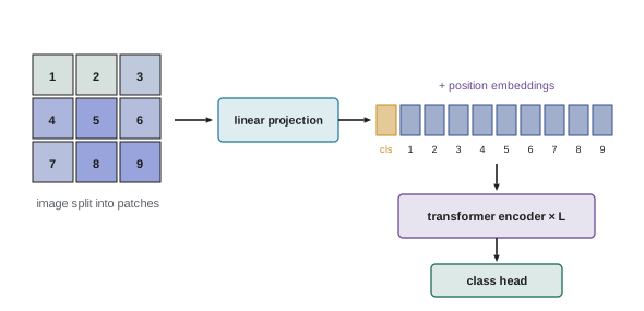
Unlike a CNN, a ViT has almost no built-in assumptions about images: no locality, no weight sharing across positions beyond the patch projection, and only weak translation equivariance. Every patch can relate to every other from the first layer, giving a global receptive field. The cost of weak inductive bias is data hunger: trained only on ImageNet's 1.3 million images, the original ViT underperformed comparable CNNs, but pretrained on hundreds of millions of images it outperformed them. Later work (DeiT) showed that strong augmentation, regularization and distillation from a CNN teacher allow ViTs to train well on ImageNet alone. Hierarchical transformers such as the Swin Transformer reintroduce locality by computing attention within shifted local windows and merging patches between stages, producing CNN-like feature pyramids that suit detection and segmentation.

Cost of vision transformers

Self-attention cost grows with the square of the number of tokens, and the number of tokens grows with the square of image resolution, so attention cost grows with the fourth power of resolution.

# Vision Transformer (ViT-Base): patch size 16, width 768, 12 layers, 12 heads, MLP 3072
d, layers, mlp, patch = 768, 12, 3072, 16
per_layer = 4 * d * d + 2 * d * mlp            # attention projections + MLP (biases and norms ignored)
patch_embed = patch * patch * 3 * d
print(f"parameters: {(layers * per_layer + patch_embed) / 1e6:.1f} M  (patch embedding {patch_embed / 1e6:.2f} M)")
for res in (224, 384, 512, 1024):
    n = (res // patch) ** 2 + 1                # patches plus a class token
    dense = 2 * layers * per_layer * n         # multiply-adds x 2 for the weight matrices
    attn = 2 * layers * 2 * n * n * d          # QK^T and attention x V
    print(f"{res:4d} px: {n:5d} tokens, {(dense + attn) / 1e9:7.1f} GFLOPs, attention share {attn / (dense + attn) * 100:4.1f}%")

parameters: 85.5 M  (patch embedding 0.59 M)
 224 px:   197 tokens,    34.9 GFLOPs, attention share  4.1%
 384 px:   577 tokens,   110.3 GFLOPs, attention share 11.1%
 512 px:  1025 tokens,   212.8 GFLOPs, attention share 18.2%
1024 px:  4097 tokens,  1314.7 GFLOPs, attention share 47.1%

ViT-Base has about 86 million parameters, almost all in its transformer blocks. At 224 pixels it processes 197 tokens with about 35 billion floating-point operations (17.5 billion multiply-adds), of which attention is only 4%. At 1024 pixels, needed for detection of small objects or reading fine text, there are 4097 tokens, the computation rises 38-fold, and attention becomes almost half the cost. High-resolution vision therefore relies on larger patches, windowed or hierarchical attention, token merging and pruning, or processing images as several tiles, as many multimodal language models do.

Self-supervised learning

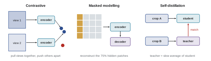
Labelled data is expensive, but unlabelled images are abundant. Self-supervised learning creates a training signal from the images themselves, so models can learn general visual features from hundreds of millions of images without labels. Three families dominate:

• Contrastive learning (SimCLR, MoCo, 2020): create two differently augmented views of each image (crops, colour changes, blur) and train an encoder so that the two views of the same image have similar embeddings while views of different images are dissimilar. The model must learn what stays the same under augmentation, which turns out to be the image's content.
• Masked image modelling (BEiT, MAE, 2021): hide a large fraction of image patches (MAE masks 75%) and train the model to reconstruct them from the visible ones, analogous to BERT's masked language modelling. Because the encoder sees only the visible quarter of patches, MAE pretraining is efficient.
• Self-distillation (DINO, 2021; DINOv2, 2023): a student network learns to match the output of a teacher network (a slowly updated average of the student) on different views of the same image, without negative pairs. DINO features turned out to separate objects from backgrounds without ever seeing a segmentation label, and DINOv2, trained on 142 million curated images, produces features that work well for classification, segmentation and depth estimation with only a simple trained head.

Self-supervised models are evaluated by linear probing (training only a linear classifier on frozen features), k-nearest-neighbour classification using the features, and fine-tuning on downstream tasks.

Contrastive vision-language models

In 2021, OpenAI's CLIP trained an image encoder and a text encoder together on 400 million image-caption pairs collected from the web. For a batch of \(N\) pairs, each image should be most similar to its own caption and each caption to its own image. The similarity of every image with every caption is computed as a scaled cosine similarity, and a symmetric cross-entropy loss (InfoNCE) rewards the correct pairs:

where \(s_{ij}\) is the cosine similarity of image \(i\) and caption \(j\) and \(\tau\) is a temperature (learned in CLIP).

import numpy as np

rng = np.random.default_rng(0)
# toy image and text embeddings for 4 matching pairs (CLIP-style), unit length, dimension 32
concepts = rng.normal(size=(4, 32))
img = concepts + 0.6 * rng.normal(size=(4, 32))
txt = concepts + 0.6 * rng.normal(size=(4, 32))
img /= np.linalg.norm(img, axis=1, keepdims=True); txt /= np.linalg.norm(txt, axis=1, keepdims=True)

def info_nce(img, txt, tau):
    logits = img @ txt.T / tau                 # similarity of every image with every caption
    logp_i = logits - np.log(np.exp(logits).sum(axis=1, keepdims=True))
    logp_t = logits.T - np.log(np.exp(logits.T).sum(axis=1, keepdims=True))
    return -(np.diag(logp_i).mean() + np.diag(logp_t).mean()) / 2, logits

np.set_printoptions(precision=2, suppress=True)
print("cosine similarities (rows: images, columns: captions):")
print(img @ txt.T)
for tau in (1.0, 0.1, 0.01):
    loss, _ = info_nce(img, txt, tau)
    print(f"temperature {tau:<5}: contrastive loss {abs(loss):.3f}")
shuffled_loss, _ = info_nce(img, txt[[1, 0, 3, 2]], 0.1)
print(f"loss with captions mismatched (temperature 0.1): {shuffled_loss:.3f}")
# zero-shot classification: pick the caption with the highest similarity
print("zero-shot predictions:", (img @ txt.T).argmax(axis=1), " correct:", np.arange(4))

cosine similarities (rows: images, columns: captions):
[[ 0.72 -0.07 -0.3   0.38]
 [-0.17  0.67  0.09 -0.03]
 [ 0.03 -0.12  0.74 -0.15]
 [ 0.19 -0.2  -0.05  0.71]]
temperature 1.0  : contrastive loss 0.895
temperature 0.1  : contrastive loss 0.012
temperature 0.01 : contrastive loss 0.000
loss with captions mismatched (temperature 0.1): 8.213
zero-shot predictions: [0 1 2 3]  correct: [0 1 2 3]

The matching pairs have cosine similarities around 0.7 and the mismatched ones near zero. With temperature 1, the softmax over these small differences is soft and the loss is 0.9; with temperature 0.1, the differences are magnified tenfold, the correct pairs dominate, and the loss falls to 0.01. Mismatching the captions raises the loss to 8.2, the signal that training uses to pull correct pairs together. Choosing the caption with the highest similarity for each image matches all four correctly, which is exactly how CLIP performs zero-shot classification.

Zero-shot classification works by writing each class as a text prompt ("a photo of a dog", "a photo of a cat") and picking the class whose text embedding is most similar to the image embedding, with no training on the target classes. CLIP matched the accuracy of a ResNet-50 trained on ImageNet without using any ImageNet training labels, and was far more robust to distribution shifts such as sketches and renditions. CLIP-style encoders (and successors such as SigLIP) now serve as the vision components of image generators, multimodal language models and image search systems.

Foundation models and how they are used

Large pretrained vision models are now the default starting point. Common patterns of use are:

• Embedding and retrieval: encode images (and text queries) into vectors for similarity search, deduplication, clustering and recommendation.
• Linear probes and light heads: train a small classifier, detector or segmentation head on frozen features with a few hundred labelled examples.
• Fine-tuning: adapt the full model, or a small number of added parameters (adapters, LoRA), for the highest accuracy on a specific domain.
• Multimodal language models: a vision encoder's patch embeddings are projected into a language model's token space, so the model can answer questions about images, read documents and charts, and describe scenes (AI-410).
• Open-vocabulary detection and segmentation: combining vision-language embeddings with detectors and promptable segmentation lets users find objects described in free text.

Data, bias and limits

Web-scale image-text data bring breadth but also problems. Captions are noisy and often describe images loosely; the data over-represent some regions, languages and groups and under-represent others; and they contain stereotypes that models absorb, so CLIP-style models have been shown to associate occupations and attributes with gender and race in biased ways. Web datasets have also been found to contain copyrighted works, private images and, in at least one widely used public dataset, links to illegal material, leading to its withdrawal for cleaning. Models trained on such data inherit these issues, so data curation, filtering, documentation (datasheets, AI-220) and evaluation for bias and safety are essential parts of building vision foundation models. Even very large models still struggle with counting, precise spatial relations, small text and fine details, and can be fooled by text written on objects (a label reading "iPod" on an apple fooled early CLIP models).

Lesson 8 turns to generative models, and Lesson 11 to the multimodal language models built on these vision encoders.