
AERO-330 · Lesson 6 of 12 · 23 min
Linearized equations of motion
Lessons 2 to 5 asked only which way the aircraft starts to move after a disturbance. To know what happens next, whether the motion dies away, oscillates or grows, and how fast, Arjun needs the equations of motion of Lesson 1 in a form he can solve. The full equations are nonlinear and coupled, but the motions that matter for stability are small departures from steady flight. Linearizing about a trimmed condition turns twelve tangled equations into two tidy sets of four linear equations, one longitudinal and one lateral-directional. Their eigenvalues are the aircraft's natural modes. This lesson builds the longitudinal set for the Tern Block 2 in cruise at 3000 m and 105 m/s .
Small perturbations
Write each variable as its steady value plus a small perturbation: \(u = u_0 + \Delta u\), \(w = 0 + \Delta w\) in stability axes, \(\theta = \theta_0 + \Delta\theta\), and so on, with the steady angular rates all zero. Substitute into the equations of Lesson 1, subtract the steady-flight balance, and drop all products of perturbations because they are second-order small. Trigonometric terms are linearized too: \(\sin(\theta_0 + \Delta\theta) \approx \sin\theta_0 + \Delta\theta\cos\theta_0\). For a symmetric aircraft in wings-level flight, something useful happens: the longitudinal variables \(u, w, q, \theta\) do not appear in the lateral equations and the lateral variables \(v, p, r, \phi\) do not appear in the longitudinal ones. The two sets decouple, which is why every textbook treats them separately.
The perturbation forces and moments are expanded in a Taylor series about the trim point, keeping only first derivatives. For example, the change in pitching moment is
Each coefficient is a dimensional stability derivative: the change in force or moment per unit change of a variable, divided by mass or by moment of inertia. They come from the non-dimensional derivatives of earlier lessons and the flight condition. For instance \(M_w = C_{m_\alpha}\,qS\bar c/(I_y u_0)\) and \(M_q = C_{m_q}(\bar c/2u_0)\,qS\bar c/I_y\). The derivative \(M_{\dot w}\) captures the lag of downwash: the tail feels the wing's change in downwash only after the air has travelled from wing to tail, which adds pitch damping.
The state-space form
Collecting terms gives four first-order equations, conveniently written as a matrix equation \(\dot{\mathbf{x}} = A\mathbf{x} + B\mathbf{u}\) with state \(\mathbf{x} = [\Delta u, \Delta w, \Delta q, \Delta\theta]^T\) and input the elevator angle:
(The perturbation symbol is dropped for clarity.) Reading the matrix row by row tells a physical story. The first row says speed changes with the drag derivative \(X_u\), with \(X_w\) as angle of attack tilts the lift and drag, and with gravity as the pitch attitude changes. The second says vertical velocity responds mainly to lift (\(Z_w\)) and to pitch rate, which rotates the velocity vector at \(u_0 q\). The third is the pitch equation: stiffness from \(M_w\) and damping from \(M_q\). The fourth says pitch attitude is the integral of pitch rate. Typical derivative magnitudes for the Tern are given in the table.
| Derivative | Meaning | Tern cruise value |
|---|---|---|
| X_u | drag change with speed | −0.0148 per s |
| Z_w | lift change with vertical velocity | −1.159 per s |
| M_w | pitch stiffness (from Cm-alpha) | −0.0807 per m s |
| M_q + M_ẇ u0 | pitch damping | −1.926 per s |
| M_δe | elevator power | −12.2 per s² per rad |
Eigenvalues are modes
With no control input, the solution of \(\dot{\mathbf{x}} = A\mathbf{x}\) is a sum of terms \(e^{\lambda t}\), where the \(\lambda\) are the eigenvalues of \(A\): the roots of the characteristic equation \(\det(\lambda I - A) = 0\). For a four-by-four matrix this is a quartic. A real root \(\lambda = -1/\tau\) gives a non-oscillatory mode that decays with time constant \(\tau\) if negative or grows if positive. A complex pair \(\lambda = -\zeta\omega_n \pm j\omega_n\sqrt{1 - \zeta^2}\) gives an oscillation with natural frequency \(\omega_n\) and damping ratio \(\zeta\). The aircraft is dynamically stable if every root has a negative real part, that is, if every root lies in the left half of the complex plane.
The corresponding eigenvectors are the mode shapes: the relative sizes and phases of \(u, w, q\) and \(\theta\) in each mode. They are what distinguish a pitching oscillation in which speed hardly changes from a slow exchange of speed and height in which angle of attack hardly changes.
# Linearized longitudinal equations of the Tern Block 2 in cruise (3000 m, 105 m/s):
# build the state matrix from the stability derivatives and find its eigenvalues.
import math
def charpoly(A):
    """Coefficients of det(sI - A), highest power first (Faddeev-LeVerrier)."""
    n = len(A); M = [[0.0] * n for _ in range(n)]; c = [1.0]
    I = [[1.0 if i == j else 0.0 for j in range(n)] for i in range(n)]
    for k in range(1, n + 1):
        AM = [[sum(A[i][l] * M[l][j] for l in range(n)) for j in range(n)] for i in range(n)]
        M = [[AM[i][j] + c[-1] * I[i][j] for j in range(n)] for i in range(n)]
        AM = [[sum(A[i][l] * M[l][j] for l in range(n)) for j in range(n)] for i in range(n)]
        c.append(-sum(AM[i][i] for i in range(n)) / k)
    return c

def roots(c, it=500):
    """All roots of a polynomial by the Durand-Kerner iteration."""
    n = len(c) - 1; a = [x / c[0] for x in c]
    z = [complex(0.4, 0.9) ** k for k in range(n)]
    for _ in range(it):
        new = []
        for i in range(n):
            p = sum(a[k] * z[i] ** (n - k) for k in range(n + 1))
            d = 1
            for j in range(n):
                if j != i: d *= (z[i] - z[j])
            new.append(z[i] - p / d)
        z = new
    return sorted(z, key=lambda r: -abs(r))

def describe(s):
    import math
    if abs(s.imag) < 1e-6:
        t = -1 / s.real if s.real < 0 else 1 / s.real
        kind = 'time constant' if s.real < 0 else 'doubles every'
        val = t if s.real < 0 else math.log(2) / s.real
        return f"real root {s.real:+.4f}: {kind} {val:.2f} s"
    wn = abs(s); z = -s.real / wn
    return f"pair {s.real:+.4f} +/- {abs(s.imag):.4f}j: wn {wn:.3f} rad/s, zeta {z:.3f}, period {2*math.pi/abs(s.imag):.1f} s"

m, Iyy, S, c, g = 6500.0, 27000.0, 28.0, 1.73, 9.81
rho, u0 = 0.909, 105.0
Q = 0.5 * rho * u0 ** 2; QS = Q * S
CL = m * g / QS; CD = 0.028 + 0.039 * CL ** 2
CLa, CDa = 5.6, 2 * 0.039 * CL * 5.6
Cma, Cmq, Cmad = -1.00, -20.0, -6.0          # per radian (Cmq, Cmad on q c/2u0 and alpha-dot c/2u0)
print(f"q = {Q:.0f} Pa, CL = {CL:.3f}, CD = {CD:.4f}")
# dimensional derivatives (Nelson notation), per unit of u, w (m/s) and q (rad/s)
Xu = -2 * CD * QS / (m * u0)
Xw = (CL - CDa) * QS / (m * u0)
Zu = -2 * CL * QS / (m * u0)
Zw = -(CLa + CD) * QS / (m * u0)
Mw = Cma * QS * c / (Iyy * u0)
Mwd = Cmad * (c / (2 * u0)) * QS * c / (Iyy * u0)
Mq = Cmq * (c / (2 * u0)) * QS * c / Iyy
A = [[Xu, Xw, 0.0, -g],
     [Zu, Zw, u0, 0.0],
     [Mwd * Zu, Mw + Mwd * Zw, Mq + Mwd * u0, 0.0],
     [0.0, 0.0, 1.0, 0.0]]
print("state x = [u, w, q, theta]; A =")
for row in A: print("  " + "  ".join(f"{v:+9.4f}" for v in row))
cp = charpoly(A)
print("characteristic polynomial:", "  ".join(f"{v:+.4f}" for v in cp))
for s in roots(cp):
if s.imag >= -1e-9: print(" " + describe(s))q = 5011 Pa, CL = 0.454, CD = 0.0361
state x = [u, w, q, theta]; A =
-0.0148 +0.0526 +0.0000 -9.8100
-0.1869 -1.1586 +105.0000 +0.0000
+0.0008 -0.0807 -1.9255 +0.0000
+0.0000 +0.0000 +1.0000 +0.0000
characteristic polynomial: +1.0000 +3.0990 +10.7616 +0.1810 +0.1569
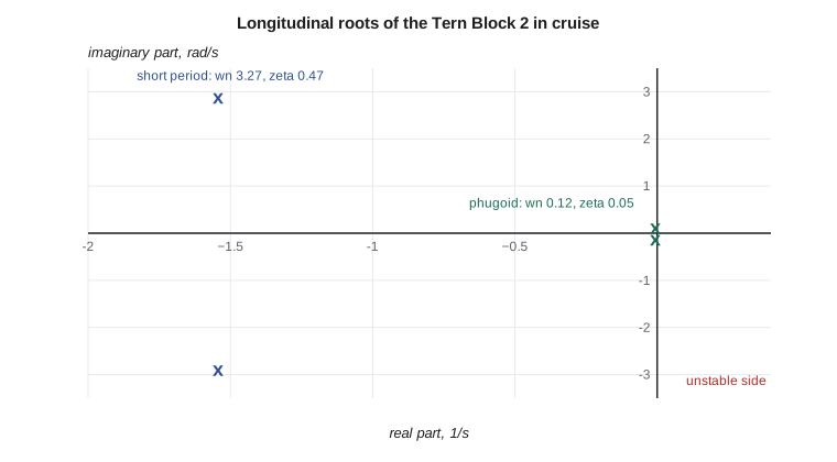
pair -1.5432 +/- 2.8856j: wn 3.272 rad/s, zeta 0.472, period 2.2 s
pair -0.0063 +/- 0.1209j: wn 0.121 rad/s, zeta 0.052, period 52.0 sThe program finds the characteristic quartic and its four roots. They come as two complex pairs, as they almost always do for a conventional aircraft. The first pair, \(-1.54 \pm 2.89j\), has a natural frequency of 3.27 rad/s and a damping ratio of 0.47: a fast, well-damped pitching motion with a period of about 2 seconds. The second, \(-0.0063 \pm 0.121j\), has a natural frequency of 0.12 rad/s, a period of 52 seconds and a damping ratio of only 0.05. These are the short-period mode and the phugoid, the two longitudinal modes that Lesson 7 studies in detail. All four roots have negative real parts, so the Tern is dynamically stable in cruise.
Why solve it this way
Engineering tools find eigenvalues with the QR algorithm, which is faster and more robust than forming the characteristic polynomial. The program uses the polynomial route because it shows each step and needs nothing beyond standard Python. For four-by-four systems with well-separated roots it is accurate; for larger or badly scaled matrices, forming the polynomial loses precision, and professional tools avoid it. The program's coefficients also allow a classical check called Routh's criterion: for a quartic with all coefficients positive, the system is stable if \(c_1c_2c_3 > c_3^2 + c_1^2c_4\). For the Tern, \(3.099 \times 10.76 \times 0.181 = 6.04\) comfortably exceeds \(0.181^2 + 3.099^2 \times 0.157 = 1.54\). The same test can be applied with the derivatives as symbols to find exactly which combination of them would make the phugoid unstable.
Linear models have limits worth stating. They are valid for small perturbations about one flight condition. Near the stall, where lift no longer varies linearly with angle of attack, or in large manoeuvres where the products of rates matter, the full nonlinear equations must be used. The Tern's simulator therefore runs the full twelve-state model with tabulated aerodynamic data, and the linear models are extracted from it at many flight conditions for stability analysis and control design.
Worked problem
Reading a root
A mode has eigenvalues \(-0.8 \pm 2.4j\). Find its natural frequency, damping ratio and period.
Show solution
- \(\omega_n = \sqrt{0.8^2 + 2.4^2} = 2.53\) rad/s.
- \(\zeta = 0.8/2.53 = 0.316\).
- Period \(= 2\pi/2.4 = 2.62\) s.
Answer: The amplitude halves every \(\ln 2/0.8 = 0.87\) s, so it is mostly gone within two cycles.
Worked problem
Building a derivative
At 100 m/s and dynamic pressure 5000 Pa, an aircraft with \(S = 30\) m², \(\bar c = 1.8\) m and \(I_y = 30\,000\) kg m² has \(C_{m_\alpha} = -1.1\) per radian. Find \(M_w\).
Show solution
- \(M_\alpha = -1.1 \times 5000 \times 30 \times 1.8/30\,000 = -9.9\) per s².
- \(M_w = M_\alpha/u_0 = -0.099\) per m s.
Answer: The short-period frequency is roughly the square root of −M_α plus a damping term, so this aircraft's short period will be near 3 rad/s.
Common mistakes
MistakeKeeping products of perturbations in a linear model.
InsteadSmall-perturbation theory drops them; they belong in the nonlinear simulator.
MistakeCalling the aircraft stable because the static margin is positive.
InsteadDynamic stability needs every eigenvalue in the left half-plane.
MistakeConfusing damped frequency with natural frequency.
InsteadThe oscillation frequency is ω_n√(1 − ζ²); the period uses it.
MistakeUsing a linear model far from its trim point.
InsteadRe-linearize at each flight condition; near the stall use the nonlinear model.
Summary and key terms
- Linearizing the equations of motion about a trimmed, wings-level flight condition separates them into longitudinal and lateral-directional sets.
- Forces and moments are expanded with dimensional stability derivatives, giving a state-space model x-dot = Ax + Bu.
- The eigenvalues of A are the natural modes: real roots for non-oscillatory modes, complex pairs for oscillations with a natural frequency and damping ratio.
- The aircraft is dynamically stable when every root lies in the left half-plane.
- For the Tern in cruise the longitudinal roots are a well-damped short period and a lightly damped phugoid.
- Small perturbation
- A departure from trimmed flight small enough for products to be neglected.
- Dimensional derivative
- A force or moment derivative divided by mass or inertia, used in the state matrix.
- State-space model
- A set of first-order equations x-dot = Ax + Bu.
- Eigenvalue
- A root of det(λI − A) = 0, describing one mode.
- Natural frequency
- ω_n, the magnitude of a complex root.
- Damping ratio
- ζ, minus the real part divided by the natural frequency.
- Routh criterion
- An algebraic test of the characteristic polynomial for stability.
Practice problems
Work each problem on paper first, then reveal the answer to check.
Why do the longitudinal and lateral equations separate?
Show answer
For a symmetric aircraft in wings-level flight, the cross-coupling terms vanish after linearization.
What does M_ẇ represent physically?
Show answer
The lag of downwash reaching the tail, which adds pitch damping.
In the program, make Cm_alpha −0.2. What happens to the short period?
Show answer
Its frequency falls and its damping rises; the two roots may approach the real axis.
What is the period of a mode with roots −0.1 ± 0.5j?
Show answer
2π/0.5 = 12.6 s.
State the condition for dynamic stability in terms of eigenvalues.
Show answer
Every eigenvalue has a negative real part.
Why do professional tools avoid forming the characteristic polynomial?
Show answer
It loses precision for large or badly scaled matrices; QR is more robust.
Lesson quiz · 5 questions
Score 60% or more to complete this lesson.
Create a free account to save your progress, take quizzes and earn a certificate.