
ACCT-421 · Lesson 5 of 12 · 27 min
Linear programming and shadow prices
The ranking rule from lesson 4 works when one resource is scarce. Real plants usually face several constraints at once: paint hours, welding hours, assembly hours, supplies of steel, minimum quantities promised to customers and maximum quantities the market will take. When more than one constraint can bind, ranking by contribution per unit of a single resource no longer guarantees the best answer. Linear programming (LP) solves this more general problem. This lesson shows how to formulate a product mix problem as a linear program, solve it graphically for two products and with software for more, and interpret the results that matter most to managers: shadow prices, slack and the ranges over which they hold. It ends with the limitations that the management accountant must explain when presenting an LP answer.
Formulating a linear program
A linear program has three parts. Decision variables are the quantities to be chosen, such as the number of each product to make. The objective function is the quantity to be maximized or minimized, such as total contribution, written as a linear combination of the decision variables. Constraints are linear inequalities that limit the decision variables, such as the hours available on a machine or the maximum demand for a product. The word linear means that every relationship is proportional: doubling output doubles the hours used and doubles the contribution.
For Northgate's Farm Systems plant, Grace defines three decision variables: the numbers of Auger A10 units (A), Conveyor C8 units (C) and Bin sweep S3 units (S) to make next year. The objective is to maximize contribution, using the contribution per unit from lesson 4. The constraints are the hours of paint, welding and assembly available, the tonnes of steel the plant's supplier has committed to deliver, minimum quantities promised to key dealers, and maximum demand.
The lower bounds on augers and conveyors reflect commitments in Northgate's dealer agreements: key dealers are guaranteed a minimum allocation. The upper bounds are the demand estimates from the sales plan. Getting the formulation right is most of the work. Each coefficient has to come from a reliable source, such as engineering standards for hours and bills of materials for steel, and each constraint must reflect a real limit rather than a convenient assumption.
The graphical method for two products
With two decision variables, an LP can be solved by drawing it. Each constraint is a straight line dividing the possible combinations into those that satisfy it and those that do not. The combinations that satisfy every constraint form the feasible region, a polygon. The objective function can be drawn as a family of parallel iso-contribution lines, each showing combinations that earn the same contribution. The optimal solution is the corner of the feasible region touched by the highest iso-contribution line. A fundamental result of linear programming is that if an optimum exists, at least one corner point is optimal, so one approach is to calculate contribution at every corner and pick the largest.
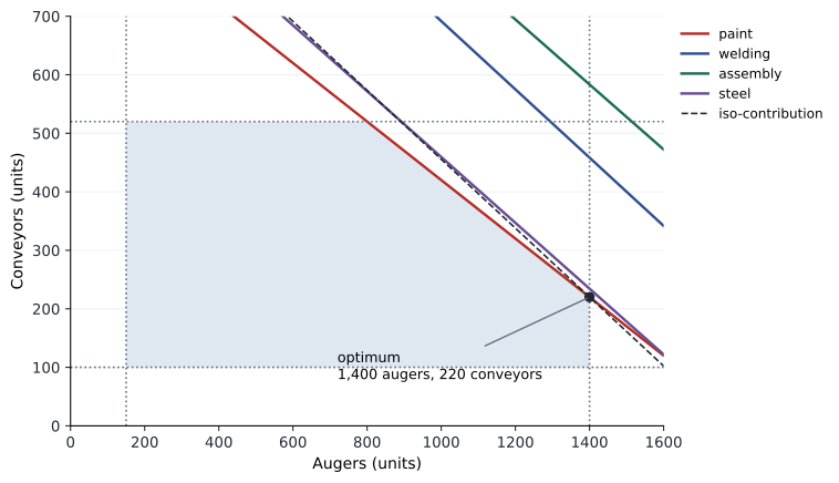
Grace fixes bin sweeps at their demand limit of 1,900, which uses 1,520 paint hours, and draws the problem for augers and conveyors. The remaining 3,680 paint hours form a line from 1,840 augers with no conveyors to 920 conveyors with no augers. The auger demand limit of 1,400 cuts across it, and so does the conveyor demand limit of 520. The corner where auger demand meets the paint constraint gives 1,400 augers and 220 conveyors, the same mix lesson 4 found by ranking. The graph also shows something the ranking could not: the steel constraint lies very close to that corner, which means a small change in paint hours might make steel binding instead.
Solving with software
Practical LP problems have many variables and constraints and are solved with software. Spreadsheet solvers handle small problems; dedicated optimization libraries handle large ones. Grace uses the open-source HiGHS solver through Python's SciPy library, which also reports the shadow prices she needs.
# Product mix by linear programming with several constraints (invented data).
import numpy as np
from scipy.optimize import linprog

names = ['Auger A10', 'Conveyor C8', 'Bin sweep S3']
cm = np.array([1590, 2700, 1060])            # contribution per unit, from lesson 4
#                 A10   C8    S3      limit
A = np.array([[2.0,  4.0,  0.8],      # paint line hours        5,200
              [3.5,  6.0,  1.5],      # welding hours          10,500
              [5.0,  9.0,  2.5],      # assembly hours         17,000
              [0.9,  1.6,  0.35]])    # steel (t)              2,300
b = np.array([5200, 10500, 17000, 2300])
labels = ['paint hours', 'welding hours', 'assembly hours', 'steel (t)']
bounds = [(150, 1400), (100, 520), (0, 1900)]   # dealer commitments and market demand

res = linprog(-cm, A_ub=A, b_ub=b, bounds=bounds, method='highs')
x = res.x
print('Optimal plan:', {n: round(v) for n, v in zip(names, x)})
print(f"Total contribution: {-res.fun:,.0f}")
for lab, used, cap, dual in zip(labels, A @ x, b, res.ineqlin.marginals):
    print(f"  {lab:15s} used {used:8,.0f} of {cap:7,}  shadow price {-dual:7.2f} per unit")
# check one shadow price by re-solving with 100 more paint hours
b2 = b.copy(); b2[0] += 100
res2 = linprog(-cm, A_ub=A, b_ub=b2, bounds=bounds, method='highs')
print(f"Extra contribution from 100 more paint hours: {(-res2.fun) - (-res.fun):,.0f}")
# reduced costs on the bounds tell us which demand limits bind
for n, lo, up in zip(names, res.lower.marginals, res.upper.marginals):
print(f" {n:13s} value of one more unit of demand: {-up:7.2f}")Optimal plan: {'Auger A10': 1400, 'Conveyor C8': 220, 'Bin sweep S3': 1900}
Total contribution: 4,834,000
paint hours used 5,200 of 5,200 shadow price 675.00 per unit
welding hours used 9,070 of 10,500 shadow price 0.00 per unit
assembly hours used 13,730 of 17,000 shadow price 0.00 per unit
steel (t) used 2,277 of 2,300 shadow price 0.00 per unit
Extra contribution from 100 more paint hours: 38,812
Auger A10 value of one more unit of demand: 240.00
Conveyor C8 value of one more unit of demand: -0.00
Bin sweep S3 value of one more unit of demand: 520.00The solver confirms the mix of 1,400 augers, 220 conveyors and 1,900 bin sweeps, with contribution of 4,834,000 dollars. Only the paint line is fully used. Welding has 1,430 hours of slack, assembly 3,270 hours, and steel 23 tonnes, a narrow margin. Augers and bin sweeps are at their demand limits.
Shadow prices
The shadow price of a constraint is the change in the optimal objective value from one more unit of the constrained resource, holding everything else constant. It is also called the dual price or marginal value. Constraints with slack have a shadow price of zero: an extra welding hour is worthless when 1,430 are already unused. The binding paint constraint has a shadow price of 675 dollars an hour, the contribution per paint hour of the marginal product, the conveyor, which matches lesson 4.
Shadow prices answer practical questions directly. What is the most Northgate should pay for an extra hour of paint capacity, through overtime, a rented booth or outsourcing? Up to 675 dollars above the normal cost of that hour. Is it worth paying a premium for extra welding hours or steel at the moment? No. The reduced costs on the demand limits answer a related question: an extra unit of bin sweep demand is worth 520 dollars, and an extra auger 240 dollars, because each would displace some conveyor production on the paint line. Those values guide where the sales team should push hardest.
| Constraint | Used | Available | Slack | Shadow price |
|---|---|---|---|---|
| Paint hours | 5,200 | 5,200 | 0 | 675 per hour |
| Welding hours | 9,070 | 10,500 | 1,430 | 0 |
| Assembly hours | 13,730 | 17,000 | 3,270 | 0 |
| Steel, tonnes | 2,277 | 2,300 | 23 | 0 |
| Auger demand | 1,400 | 1,400 | 0 | 240 per unit |
| Bin sweep demand | 1,900 | 1,900 | 0 | 520 per unit |
The range of validity
A shadow price holds only over a range. As more of a resource is added, the optimal mix changes, and eventually another constraint binds and the shadow price changes. The program checks this directly by adding 100 paint hours and solving again. If the 675-dollar shadow price held, the extra hours would add 67,500 dollars. Instead they add only 38,812 dollars. The extra paint hours allow more conveyors, but each conveyor needs 1.6 tonnes of steel, and after about 14 more conveyors the steel constraint binds. Beyond that point, extra paint hours are worth much less, because conveyors are limited by steel.
This matters for the second paint booth proposal, which would add about 2,600 hours. Valuing those hours at 675 dollars each would suggest extra contribution of about 1.75 million a year, but that ignores both the steel limit and the conveyor demand limit of 520 units. Only 300 more conveyors could be sold, using 1,200 paint hours, and they would need 480 more tonnes of steel. Unless the steel supply can be increased, the booth's value is much lower. The proper analysis re-solves the LP with the new capacity and any other changes, which is how Grace estimates the operating profit of about 0.55 million a year after depreciation that the paint booth contributes in the capstone, having negotiated additional steel with a second supplier.
Worked problem
Using a shadow price
A contractor offers to paint conveyor frames off site for 900 dollars of extra cost per frame, freeing 3 paint hours per frame (the frames still need one hour of touch-up on Northgate's line). Is this worthwhile for a small number of frames?
Show solution
- Each outsourced frame frees 3 paint hours.
- At a shadow price of 675 dollars an hour, 3 hours are worth 2,025 dollars.
- The extra cost is 900 dollars per frame.
- Net gain per frame: 2,025 − 900 = 1,125 dollars, but only within the range where the shadow price holds; steel binds after about 14 extra conveyors.
Answer: Yes for a small number of frames, but not for hundreds unless steel supply also increases.
Sensitivity of the objective coefficients
Solvers also report how far each product's contribution can change before the optimal mix changes. For Northgate, the conveyor's contribution could rise by a modest amount before the solver would choose to make more conveyors and fewer augers, and could fall a long way before production dropped to the dealer minimum. These ranges help answer questions such as how much a steel price increase, which affects conveyors most, would have to rise before the mix should change. They are useful for planning, but they share the limitation of shadow price ranges: they hold one coefficient changing at a time.
Assumptions and limitations
Linear programming is powerful but rests on assumptions that the accountant must check and explain.
| Assumption | Meaning | When it fails |
|---|---|---|
| Linearity | Contribution and resource use are proportional to output | Volume discounts, learning effects, overtime premiums |
| Divisibility | Fractional units are acceptable | Large, indivisible items such as projects or machines |
| Certainty | All coefficients are known | Uncertain demand, prices, hours per unit |
| Independence | Products do not affect each other's demand | Dealers who buy a full range, complementary products |
| Single objective | One quantity is optimized | Strategic goals such as dealer coverage or market share |
Each assumption has a remedy. Integer programming handles indivisible items, as lesson 10's capital rationing problem shows. Non-linear relationships can sometimes be approximated with several linear pieces. Uncertainty can be explored with sensitivity analysis or simulation, as lessons 6 and 11 describe. Strategic goals can be added as constraints, as Northgate did with its dealer minimums. The most important remedy is judgment: an LP solution is a recommendation based on a model, not an instruction, and the management accountant's job is to explain what the model includes, what it leaves out and how sensitive its answer is.
Other applications
Product mix is the classic application, but LP is widely used wherever limited resources are allocated. Transportation and distribution models choose which warehouse should supply which customer to minimize freight cost. Blending models choose the cheapest mix of ingredients that meets quality specifications, a common problem in feed, fuel and chemicals. Workforce scheduling models choose shift patterns that meet demand at minimum cost. Media planning models allocate an advertising budget across channels. In each case, the formulation follows the same pattern of decision variables, a linear objective and linear constraints, and the shadow prices tell managers what an extra unit of each scarce resource is worth.
Common mistakes
MistakeRanking by one resource when several constraints can bind.
InsteadFormulate and solve a linear program with all the relevant constraints.
MistakeAssuming a shadow price holds for any amount of extra resource.
InsteadCheck the range of validity by re-solving with the change.
MistakeValuing a capacity expansion at its shadow price times the hours added.
InsteadRe-solve the model with the new capacity and any other constraints that will bind.
MistakePaying a premium for a resource with slack.
InsteadResources with slack have a shadow price of zero.
MistakePresenting an LP answer without its assumptions.
InsteadExplain linearity, divisibility, certainty and the constraints included or left out.
Summary and key terms
- A linear program has decision variables, a linear objective and linear constraints.
- The optimum lies at a corner of the feasible region; with two variables it can be found graphically.
- Northgate's optimal mix is 1,400 augers, 220 conveyors and 1,900 bin sweeps, earning 4.83 million.
- The shadow price of the paint line is 675 dollars an hour; welding, assembly and steel have slack.
- Shadow prices hold only over a range; 100 more paint hours add 38,812, not 67,500, because steel then binds.
- Reduced costs show the value of relaxing demand limits: 520 dollars per extra bin sweep sold.
- LP assumes linearity, divisibility, certainty and independence; each can be relaxed with other methods.
- An LP solution is a model-based recommendation that needs judgment and explanation.
- Linear programming
- A method for maximizing or minimizing a linear objective subject to linear constraints.
- Decision variable
- A quantity the decision maker chooses, such as units of a product.
- Feasible region
- The set of all combinations of decision variables that satisfy every constraint.
- Iso-contribution line
- A line joining combinations of products that earn the same total contribution.
- Shadow price
- The change in the optimal objective value from one more unit of a constrained resource.
- Slack
- The unused amount of a resource at the optimal solution.
- Reduced cost
- The change in the objective from forcing one more unit of a variable, or relaxing its bound.
- Integer programming
- A form of mathematical programming in which some variables must take whole-number values.
Practice problems
Work each problem on paper first, then reveal the answer to check.
What are the three parts of a linear program?
Show answer
Decision variables, an objective function and constraints.
Why is there always an optimal corner point in an LP with a solution?
Show answer
The objective is linear, so the best value on a polygon is reached at a vertex.
Which constraints bind in Northgate's optimal solution?
Show answer
Paint hours and the auger and bin sweep demand limits.
What is the most Northgate should pay above normal cost for one extra paint hour?
Show answer
675 dollars, within the valid range.
Why do 100 extra paint hours add only 38,812 dollars?
Show answer
After about 14 more conveyors the steel constraint binds, so the rest of the hours cannot be used fully.
Change steel to 2,800 tonnes in the program and re-run the 100-hour test. What happens?
Show answer
The extra hours add the full 67,500 dollars, because steel no longer binds within that range.
What is the reduced cost on bin sweep demand, and what does it mean?
Show answer
520 dollars: one more unit of bin sweep demand would raise contribution by 520.
Name two assumptions of LP that often fail in practice.
Show answer
Linearity (for example, volume discounts) and certainty of coefficients, among others.
How would you handle a decision about whole machines rather than units of product?
Show answer
Use integer programming.
Give one application of LP outside product mix.
Show answer
Transportation, blending, workforce scheduling or media planning.
Lesson quiz · 5 questions
Score 60% or more to complete this lesson.
Create a free account to save your progress, take quizzes and earn a certificate.