State feedback, pole placement and observers

PID control looks only at the output error and its derivative and integral. State-space control looks at the whole internal state of the system, positions, velocities, and for a flexible joint the twist of the transmission, and feeds back a weighted combination of all of it. With full state feedback, every closed-loop pole can be placed anywhere we like, provided the system is controllable. This is a big advantage for systems with more than two states, such as the flexible joint of lesson 3, where PD feedback from the motor angle alone cannot damp the link's oscillation. The catch is that not every state is measured. An observer, a real-time simulation of the plant corrected by the measurements, estimates the missing states. This lesson builds both halves: state feedback with pole placement, including Ackermann's formula, and the Luenberger observer, joined by the separation principle. It uses the state-space models of ROB-230.

State-space models of joints

A linear system in state-space form is \( \dot{\mathbf{x}} = \mathbf{A}\mathbf{x} + \mathbf{B}u \), \( y = \mathbf{C}\mathbf{x} \). For the rigid joint of lesson 4, choose the state \( \mathbf{x} = [q, \dot{q}]^{\mathsf{T}} \) and input \( u = \tau \):

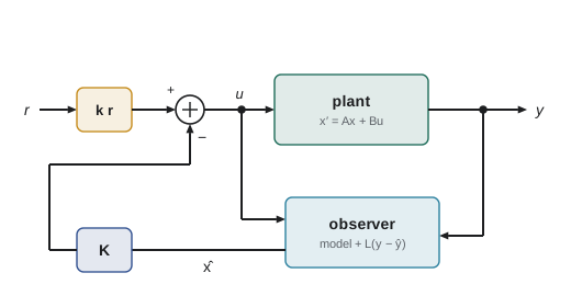
For the flexible joint, the state grows to four elements, motor angle and speed and link angle and speed, \( \mathbf{x} = [\theta_1, \dot{\theta}_1, \theta_2, \dot{\theta}_2]^{\mathsf{T}} \), with the torque acting on the motor side only. The eigenvalues of A are the open-loop poles. State feedback replaces the input with \( u = -\mathbf{K}\mathbf{x} + k_rr \), where K is a row of gains and r is the reference, giving the closed-loop dynamics

The closed-loop poles are the eigenvalues of \( \mathbf{A} - \mathbf{B}\mathbf{K} \), and choosing K to put them in chosen places is called pole placement.

Pole placement for the rigid joint

For the rigid joint, \( \mathbf{K} = [k_1, k_2] \) gives \( \mathbf{A} - \mathbf{B}\mathbf{K} = \begin{bmatrix} 0 & 1 \\ -k_1/J & -(b + k_2)/J \end{bmatrix} \) with characteristic polynomial \( s^2 + \frac{b + k_2}{J}s + \frac{k_1}{J} \). Matching this to the desired \( s^2 + 2\zeta\omega_ns + \omega_n^2 \) gives \( k_1 = J\omega_n^2 \) and \( k_2 = 2\zeta\omega_nJ - b \): exactly the PD gains of lesson 4. For a second-order plant, state feedback is PD control. Its extra power appears with more states.

Controllability

Pole placement is possible only if the input can influence every state. A system is controllable if, for any initial and final state, some input drives it from one to the other in finite time. For a system with n states, the test is the rank of the controllability matrix:

If the system is controllable, state feedback can place all n poles arbitrarily (complex poles in conjugate pairs). If it is not, some modes are untouched by the input and keep their open-loop poles whatever K is; if any of those are unstable, no controller can stabilize the system. Controllability also has a practical, graded meaning: a nearly singular \( \mathcal{C} \) means that some modes can be moved only with very large gains and torques.

Ackermann's formula

For larger systems, matching polynomial coefficients by hand is tedious. Ackermann's formula computes the gain directly for a single-input controllable system. If the desired characteristic polynomial is \( \alpha_c(s) = s^n + a_{n-1}s^{n-1} + \cdots + a_0 \), then

The formula is exact but numerically sensitive for large n; software uses more robust algorithms, but Ackermann is ideal for understanding and for small systems.

State feedback for the flexible joint

The flexible joint is where state feedback shows its value. With motor-side PD alone, the controller can damp the motor but has little influence on the link's oscillation against the transmission spring; the closed loop then has a lightly damped pair near the joint resonance that rings after every move. With all four states fed back, including the link angle and speed or equivalently the transmission twist and its rate, all four poles can be placed, so the resonant pair can be given proper damping. Industrial robots with link-side encoders or torque sensors in each joint, including most collaborative arms, use exactly this structure, often written as motor PD plus feedback of joint torque and its derivative.

Observability and the Luenberger observer

State feedback needs the whole state, but sensors measure only some of it. Velocity is usually estimated from encoder position, and on many joints the link angle is not measured at all. An observer estimates the state by running a copy of the model in parallel with the plant and correcting it with the measurement error:

Subtracting this from the plant equation gives the dynamics of the estimation error \( \mathbf{e} = \mathbf{x} - \hat{\mathbf{x}} \): \( \dot{\mathbf{e}} = (\mathbf{A} - \mathbf{L}\mathbf{C})\mathbf{e} \). Choosing the observer gain L places the eigenvalues of \( \mathbf{A} - \mathbf{L}\mathbf{C} \), so the error dies out at a chosen rate. This is the dual of pole placement, and it is possible for every pole if and only if the system is observable:

Observer poles are normally placed two to six times faster than the controller poles, so the estimate converges before the controller relies on it, but not so fast that measurement noise is amplified excessively. The Kalman filter of ROB-310 chooses L optimally given noise statistics; the Luenberger observer chooses it by pole placement.

The separation principle and integral action

When the controller uses the estimate, \( u = -\mathbf{K}\hat{\mathbf{x}} \), the combined system of plant and observer has 2n poles: the n controller poles, eigenvalues of \( \mathbf{A} - \mathbf{B}\mathbf{K} \), and the n observer poles, eigenvalues of \( \mathbf{A} - \mathbf{L}\mathbf{C} \). This is the separation principle: controller and observer can be designed independently, and putting them together does not move either set of poles. It holds exactly for linear models; with model error it holds approximately, which is one reason to keep observer and controller poles well separated.

State feedback, like PD control, leaves a steady error under a constant disturbance. The cure is to add an integral state \( x_I = \int (r - q)\,dt \) to the state vector and place the poles of the augmented system, \( u = -\mathbf{K}\mathbf{x} + k_Ix_I \). For the rigid joint this produces exactly the PID structure of lesson 4, with all three poles placed at once.

Numerical design for the flexible joint

The code below builds the four-state flexible-joint model of lesson 3, checks controllability with the motor torque as input and observability with only the motor encoder as output, and uses Ackermann's formula to place all four closed-loop poles: a pair representing the gross motion and a well-damped pair near the resonance.

import numpy as np
J1, J2, k, c = 1.2, 0.78, 3.0e4, 5.0                # joint-side values from lesson 3
A = np.array([[0, 1, 0, 0],
              [-k/J1, -c/J1, k/J1, c/J1],
              [0, 0, 0, 1],
              [k/J2, c/J2, -k/J2, -c/J2]])
B = np.array([[0], [1/J1], [0], [0]])
C = np.array([[1, 0, 0, 0]])                          # motor encoder only
Ctrb = np.hstack([np.linalg.matrix_power(A, i) @ B for i in range(4)])
Obsv = np.vstack([C @ np.linalg.matrix_power(A, i) for i in range(4)])
print("rank controllability:", np.linalg.matrix_rank(Ctrb), " rank observability:", np.linalg.matrix_rank(Obsv))
print("open-loop poles:", np.round(np.linalg.eigvals(A), 1))
wn1, z1, wn2, z2 = 30.0, 1.0, 250.0, 0.5            # desired: slow pair and damped resonance pair
coef = np.polymul([1, 2*z1*wn1, wn1**2], [1, 2*z2*wn2, wn2**2])
alpha = sum(cf*np.linalg.matrix_power(A, 4 - i) for i, cf in enumerate(coef))
K = np.array([[0, 0, 0, 1]]) @ np.linalg.inv(Ctrb) @ alpha
print("K =", np.round(K, 1))
print("closed-loop poles:", np.round(np.linalg.eigvals(A - B @ K), 1))

rank controllability: 4  rank observability: 4
open-loop poles: [-5.3+251.9j -5.3-251.9j  0.   +0.j  -0.   +0.j ]
K = [[ 17133.     359.3 -15378.    -235.6]]
closed-loop poles: [-125.+216.5j -125.-216.5j  -30.  +0.j   -30.  -0.j ]

Both matrices have full rank, so the flexible joint can be fully controlled with motor torque and fully observed, in principle, from the motor encoder alone. The open-loop poles show the rigid-body pair at the origin and the lightly damped resonance near 252 rad/s; after feedback, the resonance pair has damping ratio 0.5. The gains reveal the structure: nearly equal and opposite weights on the motor and link angles (about 17,100 and −15,400 N·m/rad) amount to strong feedback of the transmission twist \( \theta_1 - \theta_2 \), with a net position gain of only about 1,750 N·m/rad, and the speed gains likewise act mostly on the twist rate. In practice those link states would be measured by a link encoder or estimated by an observer, since estimating them from the motor encoder alone is possible but sensitive to model error.