
ROB-300 · Lesson 5 of 12 · 33 min
Stability analysis of control loops
A controller that makes the robot faster but unstable is worse than useless; it is dangerous. Stability analysis tells us, before we touch the hardware, whether a loop will settle, how much gain we can add before it oscillates, and how much unmodeled delay or lag it can tolerate. ROB-230 introduced poles, Bode plots and gain and phase margins. This lesson adds the classical tools engineers use to analyze closed loops as a gain changes: the Routh–Hurwitz criterion, which tests stability from polynomial coefficients without finding roots; the root locus, which shows how closed-loop poles move as gain rises; and the Nyquist criterion, which connects open-loop frequency response to closed-loop stability and justifies the margins. Each is applied to the joint loops of lesson 4.
Stability of a closed loop
A linear time-invariant closed loop is stable when all roots of its characteristic polynomial, the closed-loop poles, have negative real parts. For a unity-feedback loop with controller C(s) and plant P(s), the characteristic equation is
where L(s) is the loop transfer function. Writing \( L(s) = KN(s)/D(s) \), the closed-loop poles are the roots of \( D(s) + KN(s) = 0 \). For a first or second-order polynomial with all coefficients positive, stability is automatic. From third order up it is not, which is why PID loops on joints with lags, and any loop with delay, need analysis.
The Routh–Hurwitz criterion
Routh's 1877 method decides how many roots of a polynomial lie in the right half-plane using only arithmetic on the coefficients. For \( a_ns^n + a_{n-1}s^{n-1} + \cdots + a_0 \), a necessary condition is that all coefficients be present and have the same sign. To test sufficiency, build the Routh array: the first two rows hold alternate coefficients, and each later entry is computed from the two rows above by
The number of sign changes in the first column equals the number of roots in the right half-plane. For a cubic \( a_3s^3 + a_2s^2 + a_1s + a_0 \) with positive coefficients, the array reduces to a single condition:
which is the PID stability condition \( (b + K_d)K_p > JK_i \) quoted in lesson 4. The real strength of the method is that it handles symbolic gains, so it gives the range of a gain for which a loop is stable.
Worked problem
Stable gain range for a joint with a lag
A joint position loop has a proportional controller K and a plant that includes the motor-drive lag and a velocity filter, giving \( L(s) = K/(s(s + 2)(s + 5)) \). Find the range of K for stability and the frequency of oscillation at the limit.
Show solution
- Characteristic polynomial: \( s(s + 2)(s + 5) + K = s^3 + 7s^2 + 10s + K \).
- Cubic condition: \( 7 \times 10 > 1 \times K \), so K < 70; also K > 0.
- At K = 70 the \( s^1 \) row of the Routh array is zero, and the auxiliary polynomial from the \( s^2 \) row is \( 7s^2 + 70 = 0 \), giving \( s = \pm j\sqrt{10} \).
Answer: Stable for 0 < K < 70. At K = 70 the loop oscillates at \( \sqrt{10} \approx 3.16 \) rad/s (period about 2.0 s). These are exactly the ultimate gain and period that a Ziegler–Nichols experiment would measure, found here without running the robot.
Worked problem
Routh test on a fourth-order loop
Test \( s^4 + 3s^3 + 3s^2 + 2s + 4 \) for stability.
Show solution
- Rows: \( s^4 \): 1, 3, 4; \( s^3 \): 3, 2.
- \( s^2 \): \( (3 \times 3 - 1 \times 2)/3 = 2.333 \), and \( (3 \times 4 - 0)/3 = 4 \).
- \( s^1 \): \( (2.333 \times 2 - 3 \times 4)/2.333 = (4.667 - 12)/2.333 = -3.14 \).
- \( s^0 \): 4. First column 1, 3, 2.333, −3.14, 4 has two sign changes.
Answer: Unstable, with two roots in the right half-plane, even though every coefficient is positive. Positive coefficients are necessary but not sufficient beyond second order.
The root locus
Routh tells us whether the loop is stable; the root locus shows how the closed-loop poles move as a gain K rises from zero to infinity, so we can choose K for the response we want. Evans' rules, published in 1948, let us sketch the locus by hand for \( L(s) = KN(s)/D(s) \) with n poles and m zeros:
- The locus starts (K = 0) at the open-loop poles and ends (K → ∞) at the open-loop zeros, or at infinity along asymptotes for the n − m poles that have no zero to reach.
- Points on the real axis lie on the locus if an odd number of real poles and zeros lie to their right.
- The asymptotes leave from the centroid \( \sigma_a = (\sum p_i - \sum z_i)/(n - m) \) at angles \( (2k + 1)180°/(n - m) \).
- Branches leave the real axis at breakaway points, where \( dK/ds = 0 \).
- Imaginary-axis crossings, where the loop becomes unstable, are found with Routh or by substituting \( s = j\omega \).
Worked problem
Sketching a root locus
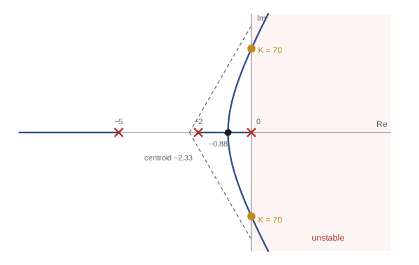
Sketch the root locus of \( L(s) = K/(s(s + 2)(s + 5)) \).
Show solution
- Three poles (0, −2, −5), no zeros: three branches, all going to infinity.
- Real-axis segments: between 0 and −2 (one pole to the right) and left of −5 (three poles to the right).
- Asymptotes: centroid \( (0 - 2 - 5)/3 = -2.33 \); angles 60°, 180°, 300°.
- Breakaway: \( K = -(s^3 + 7s^2 + 10s) \), \( dK/ds = -(3s^2 + 14s + 10) = 0 \) gives s = −0.88 (the root −3.79 is not on the locus).
- Imaginary crossing at \( \pm j3.16 \) with K = 70, from the Routh example.
Answer: Two branches leave 0 and −2, meet at −0.88, split into a complex pair and curve toward the ±60° asymptotes, crossing the imaginary axis at K = 70. The third runs from −5 to −∞. To keep a damping ratio of about 0.5, read off the gain where the locus crosses the 60° line from the origin: roughly K = 11, giving a dominant pair near \( -0.72 \pm j1.21 \).
The root locus also shows how compensation helps. Adding a zero, as derivative action does, pulls the locus to the left and allows more gain with good damping. Adding a pole at the origin, as integral action does, pulls it to the right, which is why PID designers place the integral zero well below the crossover frequency.
The Nyquist criterion
Root locus and Routh need a polynomial model. Nyquist's criterion, from 1932, works directly with the open-loop frequency response \( L(j\omega) \), which can be measured on the robot with a sine sweep even when the model is uncertain and even when the loop contains a pure delay \( e^{-sT} \), which has no polynomial form. The Nyquist plot traces \( L(j\omega) \) in the complex plane as ω runs from −∞ to +∞. The criterion states:
where P is the number of open-loop poles in the right half-plane, N is the number of clockwise encirclements of the critical point −1 by the Nyquist plot, and Z is the number of closed-loop poles in the right half-plane. For the usual case of a stable open loop (P = 0, treating poles at the origin with a small detour), the closed loop is stable if and only if the plot does not encircle −1. The margins of ROB-230 measure how far the plot stays from −1: the gain margin is how much the gain can be multiplied before the plot reaches −1 along the negative real axis, and the phase margin is how much extra phase lag, such as delay, can be added before the point at unit magnitude rotates onto −1.
For robot control, the practical outcome is a set of design targets that keep the loop robust to modeling error: a phase margin of at least 45° and a gain margin of at least 6 dB (a factor of 2) are typical, with more margin where the plant varies a lot with payload or configuration.
Worked problem
Margins from the Routh result
For \( L(s) = K/(s(s + 2)(s + 5)) \) with K = 20, find the gain margin, and estimate the phase margin.
Show solution
- The loop goes unstable at K = 70, so the gain margin is \( 70/20 = 3.5 \), or \( 20\log_{10}3.5 = 10.9 \) dB.
- Crossover: solve \( |L(j\omega)| = 1 \): \( 20 = \omega\sqrt{\omega^2 + 4}\sqrt{\omega^2 + 25} \). Trying ω = 1.5: \( 1.5 \times 2.5 \times 5.22 = 19.6 \), close; ω ≈ 1.52 rad/s.
- Phase at crossover: \( -90° - \arctan(1.52/2) - \arctan(1.52/5) = -90° - 37.2° - 16.9° = -144.1° \).
- Phase margin: \( 180° - 144.1° = 35.9° \).
Answer: Gain margin 3.5 (10.9 dB) and phase margin about 36°. The gain margin is comfortable but the phase margin is below the usual 45° target, so the step response will overshoot about 30 %. Reducing K or adding derivative (lead) action would raise it.
Delay and the delay margin
Delays are everywhere in digital robot control: sampling and computation, communication buses, sensor processing and, for teleoperation, the network. A pure delay T leaves magnitude unchanged and adds phase lag \( \omega T \) radians, growing without limit with frequency. If a loop has phase margin \( \phi_m \) (in radians) at crossover frequency \( \omega_c \), the largest extra delay it can tolerate before instability is the delay margin
This gives a vivid design rule: faster loops, with higher crossover, tolerate proportionally less delay. A joint position loop with 20 rad/s crossover and 45° margin tolerates about 39 ms of delay; a current loop crossing over at 6,000 rad/s with the same margin tolerates only 0.13 ms, which is why current loops run in dedicated hardware next to the motor.
Worked problem
Delay margin of a joint loop
A PD-controlled joint has crossover at 25 rad/s and 60° phase margin. The controller runs at 1 kHz with one sample of computation delay and an EtherCAT bus adding 0.5 ms. Is the delay acceptable?
Show solution
- Delay margin: \( (60° \times \pi/180)/25 = 1.047/25 = 41.9 \) ms.
- Actual delay: one sample (1 ms), half a sample from the zero-order hold (0.5 ms, ROB-230), and the bus (0.5 ms): about 2 ms.
- Phase lost at crossover: \( 25 \times 0.002 = 0.05 \) rad = 2.9°.
Answer: Yes: 2 ms uses only 2.9° of the 60° margin, leaving about 57°. The same 2 ms would be serious for a loop crossing over at 500 rad/s, where it would cost 57° and nearly use up the margin.
Analyzing loops numerically
In practice engineers combine these tools with numerical computation. The code below finds closed-loop poles across a range of gains for the example loop, locates the gain at which a pole crosses the imaginary axis, and computes the gain and phase margins from the frequency response for K = 20, confirming the hand results.
import numpy as np
den = np.array([1, 7, 10, 0])             # s(s+2)(s+5)
def poles(K):
    return np.roots(den + np.array([0, 0, 0, K]))
for K in (5, 20, 60, 70, 80):
    print(f"K={K:3d}: max real part {max(poles(K).real):+.3f}")
w = np.logspace(-2, 2, 20000)
K = 20
L = K/(1j*w*(1j*w + 2)*(1j*w + 5))
mag, ph = np.abs(L), np.unwrap(np.angle(L))*180/np.pi
ic = np.argmin(abs(mag - 1)); ip = np.argmin(abs(ph + 180))
print(f"crossover {w[ic]:.2f} rad/s, phase margin {180 + ph[ic]:.1f} deg")
print(f"phase crossover {w[ip]:.2f} rad/s, gain margin {1/mag[ip]:.2f} ({-20*np.log10(mag[ip]):.1f} dB)")
print(f"delay margin {np.radians(180 + ph[ic])/w[ic]*1000:.0f} ms")K= 5: max real part -0.856 K= 20: max real part -0.561 K= 60: max real part -0.088 K= 70: max real part +0.000 K= 80: max real part +0.082 crossover 1.52 rad/s, phase margin 35.8 deg phase crossover 3.16 rad/s, gain margin 3.50 (10.9 dB) delay margin 410 ms
The largest real part crosses zero between K = 60 and 80, at 70, and the frequency-response margins agree with the hand calculation. The delay margin of about 0.4 s is large because this example loop is slow; real joint loops cross over ten to a hundred times faster.
Common mistakes
MistakeAssuming positive coefficients guarantee stability
InsteadBeyond second order, apply the full Routh test.
MistakeReading the root locus without checking which real-axis segments belong to it
InsteadUse the odd-number rule for real poles and zeros to the right.
MistakeIgnoring delay because it does not change magnitude
InsteadDelay adds phase lag \( \omega T \) and erodes phase margin.
MistakeDesigning for the nominal plant only
InsteadKeep margins of about 45° and 6 dB to cover payload and configuration changes.
MistakeAdding integral action with its zero near crossover
InsteadPlace the integral zero well below crossover to avoid losing phase margin.
Summary and key terms
- A closed loop is stable when all roots of \( 1 + L(s) = 0 \) lie in the left half-plane.
- Routh–Hurwitz counts right-half-plane roots from coefficients and gives stable gain ranges; for a cubic, \( a_2a_1 > a_3a_0 \).
- The root locus shows closed-loop poles moving from open-loop poles to zeros or infinity as gain rises.
- Evans' rules give real-axis segments, asymptotes, breakaway points and imaginary-axis crossings.
- Nyquist's criterion \( Z = N + P \) relates encirclements of −1 by \( L(j\omega) \) to closed-loop stability, and works with measured data and delays.
- Gain and phase margins measure distance from instability; typical targets are 6 dB and 45°.
- The delay margin \( \phi_m/\omega_c \) shows that faster loops tolerate less delay.
- Characteristic equation
- The equation \( 1 + L(s) = 0 \) whose roots are the closed-loop poles.
- Loop transfer function
- The product of controller and plant around the loop, L(s).
- Routh array
- A table built from polynomial coefficients whose first-column sign changes count unstable roots.
- Root locus
- The paths of closed-loop poles as a gain varies.
- Asymptote
- A straight line along which root locus branches go to infinity.
- Breakaway point
- Where locus branches leave or join the real axis.
- Nyquist plot
- The curve of \( L(j\omega) \) in the complex plane.
- Gain margin
- The factor by which loop gain can rise before instability.
- Phase margin
- The additional phase lag at crossover that would cause instability.
- Delay margin
- The largest extra time delay a loop can tolerate, \( \phi_m/\omega_c \).
Practice problems
Work each problem on paper first, then reveal the answer to check.
Is \( s^3 + 2s^2 + 3s + 4 \) stable?
Show answer
Yes; \( 2 \times 3 = 6 > 4 \).
Find the stable range of K for \( s^3 + 4s^2 + 4s + K \).
Show answer
0 < K < 16.
At the limit in the previous question, at what frequency does the loop oscillate?
Show answer
\( \sqrt{4} = 2 \) rad/s.
Where does the root locus of K/((s + 1)(s + 3)) leave the real axis?
Show answer
At s = −2, midway between the poles.
What are the asymptote angles for a loop with four poles and one zero?
Show answer
60°, 180° and 300°.
A loop has gain margin 2.5. What is that in dB?
Show answer
About 8 dB.
Crossover 50 rad/s, phase margin 50°. Find the delay margin.
Show answer
0.873/50 = 17.5 ms.
Why can Nyquist analysis use measured frequency response?
Show answer
It needs only \( L(j\omega) \), not a polynomial model.
What does derivative action do to the root locus?
Show answer
Adds a zero that pulls branches left, improving damping at higher gain.
An open loop is stable and its Nyquist plot encircles −1 once clockwise. Is the closed loop stable?
Show answer
No; Z = 1 + 0 = 1 unstable pole.
Lesson quiz · 5 questions
Score 60% or more to complete this lesson.
Create a free account to save your progress, take quizzes and earn a certificate.