Actuator dynamics and joint modeling

The manipulator equation of lesson 2 assumes that each joint torque appears exactly as commanded, at a perfectly rigid, frictionless joint. Real joints are driven by electric motors through gearboxes, belts or harmonic drives; they have friction that changes with speed and direction; they flex under load; and their motors have current, voltage and thermal limits. These effects often dominate what a controller can achieve. A position loop that would be excellent on the ideal model can limit-cycle around a target because of static friction, ring at a structural resonance it never knew existed, or saturate and wind up when the motor runs out of voltage. This lesson builds a practical joint model that adds the actuator, the transmission, friction and flexibility to the rigid-body dynamics, and shows how each affects control and motor sizing. Sensors, motor types and gear types were introduced in ROB-220; here we model their dynamics.

The electric motor as a torque source

A permanent-magnet DC or brushless motor produces torque proportional to current, \( \tau_m = k_t\,i \), and generates a back-EMF proportional to speed, \( e = k_e\,\omega_m \), with \( k_t = k_e \) in SI units. The winding obeys \( L\,di/dt + Ri + k_e\omega_m = v \). The electrical time constant \( L/R \) is typically 0.1 to 5 ms, much faster than the mechanical motion, which is why robot drives almost always run a fast inner current loop, at 10 to 40 kHz, that forces the current to follow a command. From the point of view of the position controller the motor then becomes a torque source, \( \tau_m \approx k_t\,i_{\text{cmd}} \), limited by the maximum current, and the voltage limit appears as a speed-dependent torque ceiling: at speed ω the back-EMF leaves only \( v_{\max} - k_e\omega \) to drive current through the resistance.

This torque–speed envelope is the actuator's fundamental limit. Every trajectory and controller must keep the commanded torque inside it, or the motor saturates and the closed loop no longer behaves as designed.

Gear reduction and reflected inertia

Motors are fast and weak; joints need to be slow and strong. A transmission with ratio N (motor turns per joint turn) multiplies torque by N, divides speed by N, and changes the inertia each side sees. With joint angle q and motor angle \( \theta_m = Nq \), the motor torque reaching the joint is \( \tau = \eta N\tau_m \), where η is the transmission efficiency. The kinetic energy of the motor rotor, \( \tfrac{1}{2}J_m\dot{\theta}_m^2 = \tfrac{1}{2}N^2J_m\dot{q}^2 \), shows that the rotor inertia appears at the joint multiplied by \( N^2 \). The effective inertia of a joint is therefore

For high gear ratios, the reflected rotor inertia \( N^2J_m \) can dominate the link inertia. This has two important consequences. First, the joint inertia varies much less with configuration, because the constant motor term swamps the changing \( M_{ii}(\mathbf{q}) \). Second, the coupling torques from other links, reduced by N when seen at the motor, become small disturbances. Together these explain why highly geared industrial arms can be controlled well by independent PID loops on each joint, while direct-drive and lightly geared robots need the model-based methods of lessons 9 and 10. The price of a high ratio is friction, backlash or compliance in the gearbox, poor back-drivability and the reflected inertia itself, which makes collisions harder for the robot.

An inertia-matching argument from ROB-220 suggests choosing \( N = \sqrt{J_L/J_m} \) to maximize the load acceleration for a given motor torque. At that ratio the reflected rotor inertia equals the load inertia. Real designs often depart from it to meet speed, back-drivability or cost targets.

Friction models

Friction is the largest unmodeled effect in most robot joints, and it is strongly nonlinear. The common models build up in layers:

• Coulomb friction: a constant-magnitude torque opposing motion, \( \tau_f = F_c\,\text{sign}(\dot{q}) \). It does not depend on speed but flips sign at zero velocity.
• Viscous friction: a torque proportional to speed, \( b\dot{q} \), from lubricant shear and electrical damping. It is linear and easy to compensate.
• Static friction (stiction): a breakaway torque \( F_s > F_c \) that must be exceeded before the joint starts to move.
• The Stribeck effect: as speed rises from zero, friction falls smoothly from the static level toward the Coulomb level before viscous friction takes over, because the lubricant film builds up.

A widely used static model combines them:

where \( v_s \) is the Stribeck velocity. Dynamic models such as the LuGre model add an internal state representing bristle deflection, which reproduces pre-sliding displacement and hysteresis, but the static model above already explains the main control problems.

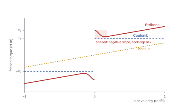
The falling part of the Stribeck curve has negative slope, which acts like negative damping: at low speeds friction decreases as speed increases, so a small speed rise reduces resistance and encourages further rise. This causes stick-slip, the jerky motion of slowly moving joints, and makes low-speed tracking difficult. Static friction also causes limit cycles under integral control. While the joint is stuck, the integrator winds up until the torque breaks friction; the joint then lurches past the target and sticks again on the other side, and the cycle repeats. Lesson 4 returns to this, and to remedies such as friction compensation and dither.

The complete rigid joint model

Combining the motor, the transmission, friction and the rigid-body dynamics, and writing everything at the joint side, each joint obeys

where \( \tau_{\text{couple},i} \) gathers the off-diagonal inertia, Coriolis and centrifugal terms from the other joints. For independent joint control (lesson 4) the coupling, the configuration-dependent part of the inertia and gravity are lumped into a disturbance, leaving a simple model: an effective inertia J and damping b driven by motor torque, with transfer function from torque to angle \( 1/(s(Js + b)) \). This is the plant that PID control is designed around.

Joint flexibility and resonance

Gearboxes, especially harmonic drives, belts, cables and torque sensors, are not perfectly stiff. A more accurate joint model has two inertias connected by a spring: the motor side \( J_1 = N^2J_m \) (referred to the joint) and the link side \( J_2 \), joined by a torsional stiffness k and damping c. With motor angle \( \theta_1 \) and link angle \( \theta_2 \), both on the joint side,

This two-mass system has a resonance at which the motor and link swing against each other, and an anti-resonance at a lower frequency:

The resonance limits the bandwidth of any loop closed through the motor encoder: pushing the loop crossover near \( \omega_r \) excites oscillation of the link that the motor encoder barely sees. A common rule keeps the position-loop bandwidth below about a third of the lowest resonance. When the encoder is on the link side, with a so-called non-collocated sensor, the loop sees the full resonance and the phase loss, and stability is harder still. Notch filters (ROB-230), input shaping and state feedback with link-side sensing (lesson 6) are the standard remedies.

Motor sizing over a duty cycle

Motors are chosen by checking three things: peak torque must lie inside the torque–speed envelope at every point of the motion; peak speed must be below the rated speed; and the RMS torque over a full cycle must not exceed the continuous rating, because winding heat grows with the square of current. The RMS torque of a cycle made of segments of torque \( \tau_k \) lasting \( t_k \) is

The torques used must be motor-side values, \( \tau_m = \tau_{\text{joint}}/(\eta N) + J_m\ddot{\theta}_m \), which include the torque to accelerate the rotor itself.

Simulating a joint with friction

The code below simulates a single geared joint, modeled as an effective inertia with Stribeck friction, driven first by a slowly rising torque to find the breakaway point and then by a constant torque, so that the speed settles where motor torque balances friction. It uses a smoothed sign function, a common numerical device to avoid chattering at zero velocity.

import numpy as np
J, Fs, Fc, vs, b = 1.5, 3.0, 2.0, 0.05, 1.5          # joint side, SI units
def friction(w):
    sgn = np.tanh(w/1e-3)                              # smooth sign near zero
    return (Fc + (Fs - Fc)*np.exp(-(w/vs)**2))*sgn + b*w
h, w, t = 1e-4, 0.0, 0.0
tau = 0.0
while w < 1e-3:                                        # ramp torque at 2 N m/s until motion starts
    tau = 2.0*t
    stuck = abs(tau) <= Fs and abs(w) < 1e-4
    w = 0.0 if stuck else w + h*(tau - friction(w))/J
    t += h
print(f"breakaway at tau = {tau:.2f} N m after {t:.2f} s")
for k in range(int(5/h)):                              # hold 3.2 N m for 5 s
    w += h*(3.2 - friction(w))/J
print(f"steady speed with 3.2 N m: {w:.3f} rad/s (expected (3.2-2.0)/1.5 = {1.2/1.5:.3f})")

breakaway at tau = 3.00 N m after 1.50 s
steady speed with 3.2 N m: 0.794 rad/s (expected (3.2-2.0)/1.5 = 0.800)

The joint stays put until the torque passes the 3.0 N·m static level, and with 3.2 N·m applied it approaches the speed where Coulomb plus viscous friction equals the drive torque, reaching within 1 % of the predicted 0.8 rad/s after five time constants \( J/b \). Simulations like this are useful for checking how a controller will behave near zero speed before trying it on hardware.