
ROB-210 · Lesson 7 of 12 · 29 min
Product of exponentials and screw theory
The Denavit–Hartenberg method needs a frame on every link, placed by careful rules. In 1984 Roger Brockett showed a different route to forward kinematics that needs only two things: the robot's tool pose at its zero configuration, and a description of each joint axis in a single fixed frame. The resulting product of exponentials (PoE) formula is built on screw theory, a nineteenth-century description of rigid motion that has become central to modern robotics. PoE is easy to set up from a CAD model, handles revolute and prismatic joints uniformly, behaves well when joint axes are nearly parallel, and leads directly to the Jacobian of lesson 10. This lesson develops the ideas from the ground up.
Rotations as exponentials
Lesson 3 introduced exponential coordinates: a rotation of angle \( \theta \) about unit axis \( \hat{\boldsymbol{\omega}} \) is captured by the vector \( \hat{\boldsymbol{\omega}}\theta \). The connection to the exponential function comes from angular velocity. A body spinning at constant angular velocity \( \hat{\boldsymbol{\omega}} \) has orientation obeying \( \dot{R} = [\hat{\boldsymbol{\omega}}]R \), where \( [\hat{\boldsymbol{\omega}}] \) is the skew-symmetric matrix of lesson 3. Like the scalar equation \( \dot{x} = ax \), this differential equation is solved by an exponential, here a matrix exponential:
The right-hand side is Rodrigues' formula again. The infinite series \( e^{A} = I + A + A^2/2! + \cdots \) collapses to three terms because the skew matrix of a unit vector satisfies \( [\hat{\boldsymbol{\omega}}]^3 = -[\hat{\boldsymbol{\omega}}] \), so the powers cycle and the sine and cosine series appear. The matrix logarithm goes the other way, from a rotation matrix back to \( \hat{\boldsymbol{\omega}}\theta \). Exponentials and logarithms are how modern software integrates gyroscope readings, interpolates orientations and measures orientation errors.
Twists and screw motions
Rigid bodies do more than rotate: they translate too. Chasles' theorem, proved in 1830, states that every rigid-body displacement can be achieved by a screw motion: a rotation about some line in space combined with a translation along the same line, like a nut turning on a bolt. The ratio of translation to rotation is the pitch of the screw. A pure rotation has zero pitch; a pure translation has infinite pitch.
A screw axis is described by a six-vector \( \mathcal{S} = (\boldsymbol{\omega}, \mathbf{v}) \). For a revolute joint, \( \boldsymbol{\omega} \) is the unit vector along the joint axis and \( \mathbf{v} = -\boldsymbol{\omega} \times \mathbf{q} \), where \( \mathbf{q} \) is any point on the axis. Physically, \( \mathbf{v} \) is the velocity that the point at the origin would have if the body rotated about the axis at unit speed. For a prismatic joint, \( \boldsymbol{\omega} = \mathbf{0} \) and \( \mathbf{v} \) is the unit vector along the direction of sliding. A screw axis scaled by a rate is a twist, the six-dimensional velocity of a rigid body, combining angular and linear velocity in one object.
| Joint type | \( \boldsymbol{\omega} \) | \( \mathbf{v} \) | Pitch |
|---|---|---|---|
| Revolute, axis through point q | Unit vector along the axis | \( -\boldsymbol{\omega} \times \mathbf{q} \) | 0 |
| Prismatic | \( \mathbf{0} \) | Unit vector along the sliding direction | Infinite |
| Helical (lead screw), pitch h | Unit vector along the axis | \( -\boldsymbol{\omega} \times \mathbf{q} + h\boldsymbol{\omega} \) | h |
Worked problem
Screw axis of a revolute joint
A joint axis is vertical, \( \boldsymbol{\omega} = (0, 0, 1) \), and passes through the point \( \mathbf{q} = (0.4, 0, 0) \) m. Find its screw axis.
Show solution
- \( \boldsymbol{\omega} \times \mathbf{q} = (0 \cdot 0 - 1 \cdot 0,\; 1 \cdot 0.4 - 0 \cdot 0,\; 0) = (0, 0.4, 0) \).
- So \( \mathbf{v} = -\boldsymbol{\omega} \times \mathbf{q} = (0, -0.4, 0) \).
- \( \mathcal{S} = (0, 0, 1,\; 0, -0.4, 0) \).
Answer: \( \mathcal{S} = (0, 0, 1, 0, -0.4, 0) \). Check: rotating at 1 rad/s about this axis, the origin, 0.4 m from it, moves at 0.4 m/s in the −y direction, which matches \( \mathbf{v} \).
The exponential of a twist
Just as a rotation is the exponential of a skew matrix, a rigid motion is the exponential of a twist. Write the twist as a 4 × 4 matrix:
Then moving along the screw axis by \( \theta \), an angle for revolute joints or a distance for prismatic ones, produces the homogeneous transform:
For a prismatic joint, with \( \boldsymbol{\omega} = \mathbf{0} \), this reduces to a pure translation by \( \mathbf{v}\theta \). The formula is exact and cheap: one Rodrigues rotation plus a 3 × 3 matrix times a vector. It is the motion a body would undergo if it moved at the constant twist \( \mathcal{S} \) for time \( \theta \).
The product of exponentials formula
Now consider a serial arm. Place the arm in its zero configuration, all joint variables zero, and let M be the tool pose in the fixed base frame in that configuration. Express each joint's screw axis \( \mathcal{S}_i \) in the base frame, also at the zero configuration. Then the forward kinematics for any joint values is:
The reasoning is elegant. Moving only the last joint by \( \theta_n \) moves the tool by \( e^{[\mathcal{S}_n]\theta_n} \) about joint n's axis, which is still where it was at zero. Then moving joint n − 1 carries joint n and the tool together about axis n − 1, which also has not moved, and so on back to the base. Because each exponential is applied about an axis that has not yet been displaced, every screw axis can be written once, at the zero configuration, in the base frame. No link frames are needed at all.
There is also a body form, in which the screw axes \( \mathcal{B}_i \) are expressed in the tool frame at zero and M appears on the left: \( T(\boldsymbol{\theta}) = M e^{[\mathcal{B}_1]\theta_1} \cdots e^{[\mathcal{B}_n]\theta_n} \). The two forms are related by the adjoint map, \( \mathcal{B}_i = [\mathrm{Ad}_{M^{-1}}]\mathcal{S}_i \), which transforms twists between frames. The space form is convenient for analysis in the base frame; the body form suits tool-centered tasks and leads to the body Jacobian.
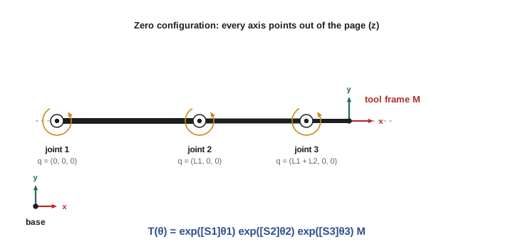
Worked example: the planar 3R arm again
Take the planar 3R arm of lesson 5 with link lengths \( L_1 \), \( L_2 \) and \( L_3 \). In the zero configuration the arm lies along the x-axis, so the tool frame has identity orientation and sits at \( (L_1 + L_2 + L_3, 0, 0) \). All joint axes point out of the plane, along z, and pass through \( (0, 0, 0) \), \( (L_1, 0, 0) \) and \( (L_1 + L_2, 0, 0) \). Using \( \mathbf{v} = -\boldsymbol{\omega} \times \mathbf{q} \):
| Joint | \( \boldsymbol{\omega} \) | Point q on axis | \( \mathbf{v} = -\boldsymbol{\omega} \times \mathbf{q} \) |
|---|---|---|---|
| 1 | (0, 0, 1) | (0, 0, 0) | (0, 0, 0) |
| 2 | (0, 0, 1) | \( (L_1, 0, 0) \) | \( (0, -L_1, 0) \) |
| 3 | (0, 0, 1) | \( (L_1 + L_2, 0, 0) \) | \( (0, -(L_1 + L_2), 0) \) |
That is the whole model: one matrix M and three six-vectors, read straight from a drawing of the arm at zero. Evaluating the product of exponentials reproduces the DH result exactly, as the code below confirms for the same joint angles as lesson 5.
import numpy as np
np.set_printoptions(precision=4, suppress=True)
def skew(w): return np.array([[0,-w[2],w[1]],[w[2],0,-w[0]],[-w[1],w[0],0]])
def exp6(S, th):
    w, v = np.array(S[:3], float), np.array(S[3:], float)
    T = np.eye(4)
    if np.allclose(w, 0):                      # prismatic
        T[:3,3] = v*th; return T
    W = skew(w)
    T[:3,:3] = np.eye(3) + np.sin(th)*W + (1-np.cos(th))*W@W
    T[:3,3] = (np.eye(3)*th + (1-np.cos(th))*W + (th-np.sin(th))*W@W) @ v
    return T
def poe(Slist, M, thetas):
    T = np.eye(4)
    for S, th in zip(Slist, thetas): T = T @ exp6(S, th)
    return T @ M
L1, L2, L3 = 0.4, 0.3, 0.1
M = np.eye(4); M[0,3] = L1 + L2 + L3
S = [(0,0,1, 0,0,0), (0,0,1, 0,-L1,0), (0,0,1, 0,-(L1+L2),0)]
T = poe(S, M, np.radians([30, 45, -60]))
print("tool position:", T[:3,3], " heading:", round(np.degrees(np.arctan2(T[1,0], T[0,0])), 1), "deg")tool position: [0.5206 0.5157 0. ] heading: 15.0 deg
The result, about (0.521, 0.516) m with a 15° heading, matches the DH calculation of lesson 5, as it must: the two methods are different parameterizations of the same geometry.
A spatial example with a prismatic joint
Consider an RRP arm: a vertical waist joint at the origin, a horizontal shoulder joint 0.5 m above the base, and a prismatic joint that extends a boom horizontally. In the zero configuration the boom points along x, and the tool sits at the end of a 0.6 m boom at \( (0.6, 0, 0.5) \).
Worked problem
Screw axes and pose of an RRP arm
Write the screw axes and find the tool position for \( \theta_1 = 90^\circ \), \( \theta_2 = 0 \), and a boom extension \( \theta_3 = 0.2 \) m.
Show solution
- Joint 1: \( \boldsymbol{\omega} = (0,0,1) \) through the origin, so \( \mathcal{S}_1 = (0,0,1,0,0,0) \).
- Joint 2: shoulder axis along y through \( (0, 0, 0.5) \), so \( \boldsymbol{\omega} = (0,1,0) \) and \( \mathbf{v} = -(0,1,0) \times (0,0,0.5) = (-0.5, 0, 0) \): \( \mathcal{S}_2 = (0,1,0,-0.5,0,0) \).
- Joint 3: prismatic along x, \( \mathcal{S}_3 = (0,0,0,1,0,0) \).
- With \( \theta_2 = 0 \), the boom extends to \( (0.8, 0, 0.5) \); then the waist turns it 90° about z to \( (0, 0.8, 0.5) \).
Answer: The tool is at (0, 0.8, 0.5) m. Note that the prismatic joint is handled exactly like the revolute ones, with no special frame rules.
Why use PoE?
PoE has practical advantages over DH. It needs no link frames, so it can be set up directly from a CAD model or a URDF by reading joint axes and positions. Revolute and prismatic joints are treated identically. Small changes in the geometry produce small changes in the screw axes, even when axes are nearly parallel, which makes PoE well suited to kinematic calibration. And the screw axes are themselves the columns of the space Jacobian, as lesson 10 shows, so velocity kinematics comes almost for free. The textbook Modern Robotics by Lynch and Park is built entirely on this approach, and its free software library implements the functions used here. DH remains common in data sheets and older controllers, so practicing engineers should be comfortable with both and able to convert between them.
| Aspect | Denavit–Hartenberg | Product of exponentials |
|---|---|---|
| Parameters per joint | 4 | 6 (screw axis), plus one M for the tool |
| Link frames needed | Yes, by strict rules | No; one base frame and the tool frame |
| Revolute versus prismatic | Different variable (θ or d) | Same formula |
| Nearly parallel axes | Parameters can jump; poor for calibration | Smooth; good for calibration |
| Link to the Jacobian | Derived separately | Screw axes give Jacobian columns directly |
| Where you meet it | Data sheets, classic texts, many controllers | Modern texts, research, calibration |
Worked problem
Checking a screw axis by its velocity
A revolute joint has \( \mathcal{S} = (0, 1, 0, -0.5, 0, 0.3) \). Find a point on its axis.
Show solution
- \( \boldsymbol{\omega} = (0,1,0) \), \( \mathbf{v} = (-0.5, 0, 0.3) \).
- A point on the axis is \( \mathbf{q} = \boldsymbol{\omega} \times \mathbf{v} \) for a unit \( \boldsymbol{\omega} \) perpendicular to \( \mathbf{v} \): \( (1 \cdot 0.3 - 0 \cdot 0,\; 0 \cdot (-0.5) - 0 \cdot 0.3,\; 0 \cdot 0 - 1 \cdot (-0.5)) = (0.3, 0, 0.5) \).
- Check: \( -\boldsymbol{\omega} \times \mathbf{q} = -(1 \cdot 0.5 - 0,\; 0 - 0,\; 0 - 1 \cdot 0.3) = (-0.5, 0, 0.3) \). Correct.
Answer: The axis is parallel to y and passes through (0.3, 0, 0.5) m. Recovering q from a screw axis is a useful sanity check when entering axes from a drawing.
Common mistakes
MistakeWriting screw axes at a non-zero configuration.
InsteadAll space-frame screw axes and M must describe the arm at its zero configuration.
MistakeGetting the sign of v wrong.
InsteadFor a revolute joint, \( \mathbf{v} = -\boldsymbol{\omega} \times \mathbf{q} \), equivalently \( \mathbf{q} \times \boldsymbol{\omega} \).
MistakePlacing M on the wrong side.
InsteadIn the space form M goes on the right; in the body form it goes on the left.
MistakeUsing a non-unit ω for a revolute joint.
InsteadNormalize the axis so θ is the joint angle in radians.
MistakeAssuming PoE and DH give different poses.
InsteadCorrectly built models of the same robot agree exactly; differences reveal an error or different zero positions.
Summary and key terms
- Rotations are matrix exponentials of skew matrices; Rodrigues' formula evaluates them.
- Every rigid displacement is a screw motion: rotation about a line plus translation along it.
- A screw axis is a six-vector (ω, v); for a revolute joint, v = −ω × q.
- The exponential of a twist gives a homogeneous transform in closed form.
- PoE forward kinematics: \( T = e^{[\mathcal{S}_1]\theta_1} \cdots e^{[\mathcal{S}_n]\theta_n} M \), with all axes at zero configuration in the base frame.
- The body form uses tool-frame axes with M on the left; the adjoint map relates the two.
- PoE needs no link frames, treats all joints alike and suits calibration and Jacobians.
- Matrix exponential
- The series \( e^{A} = I + A + A^2/2! + \cdots \), used to turn velocities into motions.
- Matrix logarithm
- The inverse of the matrix exponential, recovering a twist or rotation vector from a motion.
- Chasles' theorem
- Every rigid displacement is a rotation about a line plus a translation along it.
- Screw axis
- A six-vector (ω, v) describing a line in space and a pitch.
- Pitch
- The ratio of translation to rotation along a screw axis.
- Twist
- The six-dimensional velocity of a rigid body, combining angular and linear velocity.
- Zero configuration
- The arm pose with all joint variables equal to zero.
- Home matrix M
- The tool pose in the base frame at the zero configuration.
- Body form
- The PoE formula with screw axes expressed in the tool frame.
- Adjoint map
- The 6 × 6 matrix that transforms twists from one frame to another.
Practice problems
Work each problem on paper first, then reveal the answer to check.
What is the screw axis of a revolute joint along z through the origin?
Show answer
(0, 0, 1, 0, 0, 0).
What is the screw axis of a prismatic joint sliding along z?
Show answer
(0, 0, 0, 0, 0, 1).
A revolute axis along z passes through (0, 1, 0). Find v.
Show answer
\( -(0,0,1) \times (0,1,0) = (1, 0, 0) \).
What is the pitch of a pure rotation?
Show answer
Zero.
Why does \( e^{[\hat{\boldsymbol{\omega}}]\theta} \) need only three terms?
Show answer
Because \( [\hat{\boldsymbol{\omega}}]^3 = -[\hat{\boldsymbol{\omega}}] \), so the series folds into sine and cosine.
A planar 2R arm with \( L_1 = L_2 = 0.5 \) m lies along x at zero. Write M.
Show answer
Identity rotation with position (1.0, 0, 0).
Write \( \mathcal{S}_2 \) for that 2R arm.
Show answer
(0, 0, 1, 0, −0.5, 0).
In the space-form PoE, on which side does M appear?
Show answer
On the right.
What 6 × 6 matrix converts twists between frames?
Show answer
The adjoint map, \( [\mathrm{Ad}_T] \).
Give one advantage of PoE for calibration.
Show answer
Parameters vary smoothly even when joint axes are nearly parallel.
Lesson quiz · 5 questions
Score 60% or more to complete this lesson.
Create a free account to save your progress, take quizzes and earn a certificate.