
ROB-210 · Lesson 5 of 12 · 28 min
Denavit–Hartenberg conventions
To compute where a robot's tool is, we need the transform from each link to the next. Each such transform could be written with six arbitrary numbers, but in 1955 Jacques Denavit and Richard Hartenberg showed that, by choosing link frames cleverly, four parameters per joint are enough. Their convention became the lingua franca of robot arms: manufacturers publish DH tables, textbooks derive kinematics from them, and simulation tools import them. This lesson explains the standard and modified DH conventions, how to assign frames and read off the parameters, and how to avoid the pitfalls that make DH tables from different sources disagree.
Joints, links and the kinematic chain
A serial manipulator is a chain of rigid links connected by joints, starting at a fixed base, link 0, and ending at the last link, which carries the tool. With n joints there are n + 1 links. Joint i connects link i − 1 to link i, and it has one variable: the angle \( \theta_i \) for a revolute joint or the displacement \( d_i \) for a prismatic joint. Every joint has an axis: the line about which a revolute joint rotates or along which a prismatic joint slides. Kinematics depends only on the geometry of these axes, their directions and the distances between them, not on the shapes of the links in between.
Two lines in space are generally skew: neither parallel nor intersecting. Between any two skew lines there is exactly one common normal, the shortest line segment that is perpendicular to both. The DH convention builds each link's frame from the joint axes and these common normals, which is why four numbers suffice: two describe the relationship between consecutive joint axes, which is fixed by the link's geometry, and two describe the position along and rotation about the joint axis, one of which is the joint variable.
The standard (distal) DH convention
In the standard convention, used by Denavit and Hartenberg, by Spong and colleagues and by most manufacturers' data sheets, frame i is attached to the far (distal) end of link i, and its z-axis lies along the axis of joint i + 1. The rules are:
- \( z_i \) lies along the axis of joint i + 1.
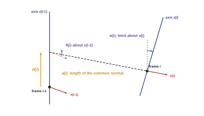
- \( x_i \) lies along the common normal from \( z_{i-1} \) to \( z_i \), pointing away from \( z_{i-1} \).
- \( y_i \) completes a right-handed frame.
- The origin of frame i is where the common normal meets \( z_i \).
With frames assigned this way, four parameters describe the transform from frame i − 1 to frame i:
| Parameter | Name | Definition | Variable for |
|---|---|---|---|
| \( \theta_i \) | Joint angle | Angle from \( x_{i-1} \) to \( x_i \), measured about \( z_{i-1} \) | Revolute joints |
| \( d_i \) | Link offset | Distance from the origin of frame i − 1 to the common normal, along \( z_{i-1} \) | Prismatic joints |
| \( a_i \) | Link length | Distance between \( z_{i-1} \) and \( z_i \), along \( x_i \) | Always fixed |
| \( \alpha_i \) | Link twist | Angle from \( z_{i-1} \) to \( z_i \), measured about \( x_i \) | Always fixed |
The transform is a product of four elementary motions, rotate about z, slide along z, slide along x, rotate about x:
Here \( c\theta_i \) means \( \cos\theta_i \) and so on. Only six of the usual twelve free numbers appear because of the clever frame choice: the x-axis is constrained to intersect and be perpendicular to the previous z-axis, which removes two degrees of freedom.
The modified (proximal) DH convention
In 1986 John Craig popularized a modified convention in which frame i is attached to the near (proximal) end of link i, with \( z_i \) along the axis of joint i itself. The parameters are the same in spirit but indexed differently, and the elementary motions occur in a different order:
The modified convention has the practical advantage that each joint's variable acts about the z-axis of the frame attached to the link it moves, which some people find more natural and which simplifies dynamics derivations. Its disadvantage is simply that it exists alongside the standard one. A DH table is meaningless unless you know which convention it uses, and the same robot has different tables in the two conventions. Fortunately the convention is usually recognizable: if the table has columns \( a_{i-1} \) and \( \alpha_{i-1} \), or if the first row has a and α equal to zero, it is probably modified.
| Feature | Standard (distal) DH | Modified (proximal) DH |
|---|---|---|
| Frame i attached to | Far end of link i | Near end of link i |
| Axis \( z_i \) lies along | Joint i + 1 | Joint i |
| Transform order | \( R_z(\theta_i)T_z(d_i)T_x(a_i)R_x(\alpha_i) \) | \( R_x(\alpha_{i-1})T_x(a_{i-1})R_z(\theta_i)T_z(d_i) \) |
| Common sources | Spong, Siciliano, most data sheets, Universal Robots | Craig, many dynamics texts, some tools |
| Tool frame | Often needs an extra fixed transform | Also needs an extra fixed transform |
Assigning frames: a procedure
Assigning DH frames is a craft that improves with practice. A reliable procedure for the standard convention is:
- Identify and draw every joint axis as an infinite line. Label them \( z_0 \) (joint 1) to \( z_{n-1} \) (joint n).
- Choose the base frame: put \( z_0 \) along joint 1 and choose \( x_0 \) conveniently, usually so that the robot's zero position has a simple form.
- For each i from 1 to n − 1, find the common normal between \( z_{i-1} \) and \( z_i \). If the axes intersect, put the origin at the intersection and make \( x_i \) perpendicular to both. If they are parallel, any common normal will do; choose one that makes \( d_i \) zero.
- Place the final frame n at the tool, with \( z_n \) usually along the approach direction, and add any fixed tool transform needed to reach the actual tool center point.
- Read off \( \theta_i \), \( d_i \), \( a_i \) and \( \alpha_i \) for each link, and mark which is the joint variable.
- Check: set all joint variables to zero, compute the tool pose and compare it with a picture or the manufacturer's zero position.
The freedom in choosing frames where axes are parallel or intersect is why different authors publish different tables for the same robot. All valid tables give the same tool pose if the zero positions and tool frames agree; they just place the intermediate frames differently.
Worked example: a planar 3R arm
The simplest useful arm has three revolute joints with parallel vertical axes, moving in a horizontal plane, with link lengths \( L_1 \), \( L_2 \) and \( L_3 \). All z-axes are parallel, so all twists are zero, and we can choose the common normals so that all offsets are zero.
| Link i | \( \theta_i \) | \( d_i \) | \( a_i \) | \( \alpha_i \) |
|---|---|---|---|---|
| 1 | \( \theta_1 \) (variable) | 0 | \( L_1 \) | 0 |
| 2 | \( \theta_2 \) (variable) | 0 | \( L_2 \) | 0 |
| 3 | \( \theta_3 \) (variable) | 0 | \( L_3 \) | 0 |
Each link transform reduces to a planar rotation by \( \theta_i \) followed by a translation \( L_i \) along the new x-axis. Multiplying the three gives the familiar result for the tool position and heading:
Here \( c_{12} \) is shorthand for \( \cos(\theta_1 + \theta_2) \), and so on. For parallel revolute axes, angles simply add, which makes planar arms easy to analyze and is why the first example of inverse kinematics in lesson 8 is the planar arm.
Worked problem
Evaluating the planar arm
A planar 3R arm has \( L_1 = 0.4 \), \( L_2 = 0.3 \) and \( L_3 = 0.1 \) m. Find the tool position and heading for \( \theta = (30^\circ, 45^\circ, -60^\circ) \).
Show solution
- Cumulative angles: \( \theta_1 = 30^\circ \), \( \theta_{12} = 75^\circ \), \( \theta_{123} = 15^\circ \).
- \( x = 0.4(0.866) + 0.3(0.259) + 0.1(0.966) = 0.346 + 0.078 + 0.097 = 0.521 \) m.
- \( y = 0.4(0.5) + 0.3(0.966) + 0.1(0.259) = 0.200 + 0.290 + 0.026 = 0.516 \) m.
- Heading: \( \phi = 15^\circ \).
Answer: The tool is at about (0.521, 0.516) m with heading 15°. The code below reproduces this by multiplying DH matrices.
Worked example: a SCARA robot
A SCARA (selective compliance assembly robot arm) has two parallel revolute joints for horizontal positioning, a prismatic joint for vertical motion and a final revolute joint to rotate the tool, all with vertical axes. It is the classic high-speed pick-and-place robot. Using the standard convention with the base frame on the floor and joint 1's axis vertical:
| Link i | \( \theta_i \) | \( d_i \) | \( a_i \) | \( \alpha_i \) |
|---|---|---|---|---|
| 1 | \( \theta_1 \) (variable) | \( h \) (column height) | \( L_1 \) | 0 |
| 2 | \( \theta_2 \) (variable) | 0 | \( L_2 \) | 180° |
| 3 | 0 | \( d_3 \) (variable) | 0 | 0 |
| 4 | \( \theta_4 \) (variable) | \( d_4 \) (tool length) | 0 | 0 |
The twist of 180° at link 2 flips the z-axis to point downward, so that a positive \( d_3 \) moves the quill down toward the work, which matches how SCARA controllers usually define the vertical axis. With that flip, the tool's height is \( h - d_3 - d_4 \) and its rotation about the vertical is \( \theta_1 + \theta_2 - \theta_4 \), because the inverted frame turns the sense of \( \theta_4 \) around.
Worked problem
SCARA tool position
A SCARA has \( h = 0.40 \), \( L_1 = 0.35 \), \( L_2 = 0.25 \) and \( d_4 = 0.10 \) m. Find the tool position for \( \theta_1 = 60^\circ \), \( \theta_2 = -30^\circ \), \( d_3 = 0.12 \) m.
Show solution
- Horizontal: \( x = 0.35\cos 60^\circ + 0.25\cos 30^\circ = 0.175 + 0.217 = 0.392 \) m.
- \( y = 0.35\sin 60^\circ + 0.25\sin 30^\circ = 0.303 + 0.125 = 0.428 \) m.
- Vertical: \( z = h - d_3 - d_4 = 0.40 - 0.12 - 0.10 = 0.18 \) m.
Answer: About (0.392, 0.428, 0.18) m. The separation of horizontal and vertical motion is what makes SCARA kinematics, and SCARA control, so simple.
DH in code
Implementing DH is a few lines. The function below builds the standard DH matrix; multiplying the matrices for each row of the table gives the forward kinematics. Writing the table as data, rather than hard-coding trigonometry, makes it easy to check against a data sheet and to reuse for different robots.
import numpy as np
np.set_printoptions(precision=3, suppress=True)
def dh(theta, d, a, alpha):
    ct, st, ca, sa = np.cos(theta), np.sin(theta), np.cos(alpha), np.sin(alpha)
    return np.array([[ct, -st*ca,  st*sa, a*ct],
                     [st,  ct*ca, -ct*sa, a*st],
                     [0,      sa,     ca,    d],
                     [0,       0,      0,    1]])
def fk(table):
    T = np.eye(4)
    for row in table: T = T @ dh(*row)
    return T
r = np.radians
planar = [(r(30), 0, 0.4, 0), (r(45), 0, 0.3, 0), (r(-60), 0, 0.1, 0)]
print("planar 3R tool position:", fk(planar)[:3, 3])
scara = [(r(60), 0.40, 0.35, 0), (r(-30), 0, 0.25, np.pi), (0, 0.12, 0, 0), (r(20), 0.10, 0, 0)]
T = fk(scara)
print("SCARA tool position:    ", T[:3, 3])
print("SCARA tool yaw (deg): ", round(np.degrees(np.arctan2(T[1,0], T[0,0])), 1))planar 3R tool position: [0.521 0.516 0. ] SCARA tool position: [0.392 0.428 0.18 ] SCARA tool yaw (deg): 10.0
The SCARA yaw printed is 60 − 30 − 20 = 10°, confirming that the downward-pointing frames reverse the sense of the last joint. Details like this are exactly why DH tables must be checked numerically before they are trusted.
Limitations and alternatives
DH parameters have known weaknesses. When two consecutive joint axes are nearly parallel, as in many arms' shoulder and elbow, a tiny manufacturing misalignment makes the common normal jump far along the axis, so the parameters change discontinuously and calibration becomes ill-conditioned. Hayati and Mirmirani proposed adding a fifth parameter, a rotation about the y-axis, for exactly this case. DH also requires frames in specific places, which may not match the CAD model or the URDF file used in ROS. URDF describes each joint with an arbitrary origin transform and an axis, which is more flexible and is what ROS tools such as robot_state_publisher and MoveIt use. The product of exponentials formula in lesson 7 avoids link frames altogether. Even so, DH remains essential knowledge, because data sheets, older literature and many controllers speak it.
Common mistakes
MistakeUsing a DH table without knowing whether it is standard or modified.
InsteadCheck the source; look for \( a_{i-1} \), \( \alpha_{i-1} \) columns that indicate the modified convention.
MistakeMeasuring \( \alpha_i \) about the wrong axis or with the wrong sign.
InsteadTwist is measured from \( z_{i-1} \) to \( z_i \) about \( x_i \) by the right-hand rule.
MistakeForgetting the joint zero offset between the DH angle and the robot's encoder zero.
InsteadAdd a constant offset column, θ = q + offset, and verify the zero position.
MistakeTreating the last DH frame as the tool center point.
InsteadAdd a fixed tool transform from the flange to the actual tool tip.
MistakeTrusting a hand-derived table without a numerical check.
InsteadEvaluate at zero and a few known poses and compare with a drawing, the controller or a simulation.
Summary and key terms
- DH parameters describe each link with four numbers: θ, d, a and α.
- Two parameters (a, α) are fixed link geometry; θ or d is the joint variable.
- Standard DH puts frame i at the far end of link i with \( z_i \) along joint i + 1; modified DH puts it at the near end.
- The standard link transform is \( R_z(\theta)T_z(d)T_x(a)R_x(\alpha) \); the modified one is \( R_x(\alpha_{i-1})T_x(a_{i-1})R_z(\theta_i)T_z(d_i) \).
- Frames are built from joint axes and their common normals; choices exist where axes are parallel or intersect.
- Planar arms have zero twists and angles that add; SCARA robots separate horizontal and vertical motion.
- DH is fragile for nearly parallel axes; URDF and product of exponentials are common alternatives.
- Serial manipulator
- A robot arm made of links connected in a single chain from base to tool.
- Joint axis
- The line about which a revolute joint rotates or along which a prismatic joint slides.
- Common normal
- The shortest segment perpendicular to two lines.
- Joint angle θ
- DH rotation about the previous z-axis; the variable of a revolute joint.
- Link offset d
- DH distance along the previous z-axis; the variable of a prismatic joint.
- Link length a
- DH distance between consecutive joint axes along their common normal.
- Link twist α
- DH angle between consecutive joint axes about the common normal.
- Modified DH
- Craig's proximal convention, with frame i on joint i.
- SCARA
- A four-axis arm with parallel vertical revolute joints and a vertical prismatic joint.
- URDF
- The XML robot description format used in ROS, with an arbitrary origin transform per joint.
Practice problems
Work each problem on paper first, then reveal the answer to check.
How many DH parameters describe each link?
Show answer
Four.
Which DH parameter is the variable of a prismatic joint?
Show answer
\( d_i \).
Two consecutive joint axes are parallel. What is their twist α?
Show answer
0° (or 180°).
Two consecutive joint axes intersect. What is the link length a?
Show answer
Zero.
Write the standard DH transform as a product of elementary motions.
Show answer
\( R_z(\theta)T_z(d)T_x(a)R_x(\alpha) \).
A planar 2R arm has \( L_1 = L_2 = 0.5 \) m and \( \theta_1 = \theta_2 = 0 \). Where is the tool?
Show answer
(1.0, 0) m.
Same arm with \( \theta_1 = 90^\circ \), \( \theta_2 = -90^\circ \). Where is the tool?
Show answer
(0.5, 0.5) m.
A SCARA has h = 0.5 m, \( d_3 = 0.2 \) m and \( d_4 = 0.05 \) m. What is the tool height?
Show answer
0.25 m.
A table has columns \( a_{i-1} \) and \( \alpha_{i-1} \). Which convention is it?
Show answer
Modified (Craig) DH.
Why do DH parameters cause calibration problems when axes are nearly parallel?
Show answer
The common normal can jump far along the axes, so parameters change discontinuously.
Lesson quiz · 5 questions
Score 60% or more to complete this lesson.
Create a free account to save your progress, take quizzes and earn a certificate.