
ROB-210 · Lesson 12 of 12 · 34 min
Mobile robot kinematics and capstone
So far the robot's base has stayed put. Mobile robots move their whole body across the floor, and their kinematics has a character of its own: wheels roll without slipping, which constrains the directions in which the robot can move at any instant, even though it can eventually reach any position and heading. This final lesson covers the kinematics of the common wheeled platforms, differential drive, car-like Ackermann steering and omnidirectional mecanum wheels, explains nonholonomic constraints, shows how wheel odometry integrates velocities into a pose, and closes with a capstone that combines a mobile base with an arm, drawing on every lesson of the course.
The pose of a mobile robot
A wheeled robot on flat ground has three degrees of freedom: position \( (x, y) \) and heading \( \theta \), an element of SE(2) as in lesson 4. Its velocity is described in its own body frame, base_link in ROS, by a forward speed \( v \), a sideways speed \( v_y \) (zero for most wheeled robots) and a turning rate \( \omega \). In ROS these appear in a geometry_msgs/Twist message on the cmd_vel topic, with linear.x, linear.y and angular.z. Converting body velocities to world velocities is a rotation by the heading:
Forward kinematics for a mobile robot is therefore a differential relationship: wheel speeds give body velocities, and body velocities must be integrated over time to give pose. Unlike an arm, there is no direct formula from wheel angles to position, because the path taken matters. Rolling the wheels forward then turning ends somewhere different from turning then rolling.
Differential drive
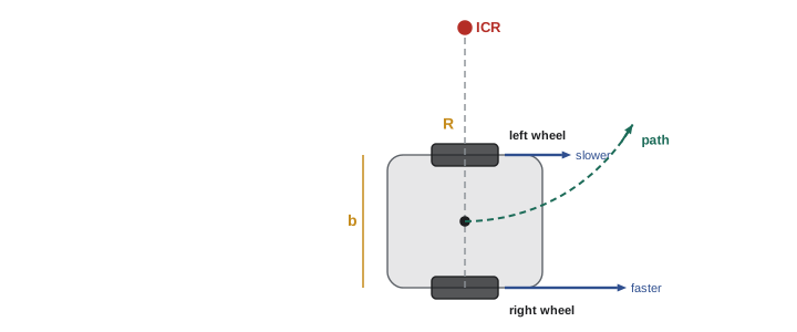
The most common mobile base has two independently driven wheels on a common axle, plus one or more passive casters. Robot vacuums, many warehouse robots and research platforms such as the TurtleBot use it. With wheel radius r, track width b (the distance between the wheels) and wheel angular speeds \( \omega_R \) and \( \omega_L \):
Equal wheel speeds drive straight; opposite speeds spin the robot on the spot; anything in between moves it along an arc about the instantaneous center of rotation (ICR), a point on the axle line at distance \( R = v/\omega \) from the robot's center. The inverse kinematics, needed to turn a commanded twist into wheel speeds, simply inverts these relations: \( \omega_R = (v + \omega b/2)/r \) and \( \omega_L = (v - \omega b/2)/r \).
Worked problem
Wheel speeds for an arc
A differential-drive robot has wheel radius 0.05 m and track width 0.30 m. It must follow an arc of radius 1.0 m to the left at 0.4 m/s. Find the wheel speeds.
Show solution
- Turn rate: \( \omega = v/R = 0.4/1.0 = 0.4 \) rad/s.
- Right wheel: \( \omega_R = (0.4 + 0.4 \times 0.15)/0.05 = 0.46/0.05 = 9.2 \) rad/s.
- Left wheel: \( \omega_L = (0.4 - 0.06)/0.05 = 6.8 \) rad/s.
- Check: \( v = 0.05(9.2 + 6.8)/2 = 0.4 \) m/s.
Answer: Right wheel 9.2 rad/s (about 88 rpm), left wheel 6.8 rad/s (about 65 rpm). The outer wheel travels a 1.15 m radius and the inner a 0.85 m radius, in the same ratio.
Nonholonomic constraints
A differential-drive robot cannot move sideways: its wheels would have to skid. Mathematically, its velocity must satisfy the rolling constraint
which says the velocity has no component perpendicular to the heading. This constraint involves velocities and cannot be integrated into a constraint on position alone, which is what makes it nonholonomic. The robot has three degrees of freedom of pose but only two of instantaneous motion. It can still reach any pose, by combining forward motion and turning, just as a driver parallel parks with a sequence of forward and backward arcs, but it cannot get there by any path it likes. This shapes planning and control: a path planner for such a robot must produce paths the robot can follow, and a controller cannot simply drive the position error to zero in a straight line. Brockett's theorem (1983) shows that no smooth, time-invariant feedback law can stabilize a nonholonomic robot to a fixed pose, which is why parking controllers use switching, time-varying or path-following strategies.
By contrast, an arm's joint limits and link geometry are holonomic constraints: they restrict where the arm can be, not how it moves between places. The distinction is one of the deep differences between manipulator and mobile robot kinematics.
Odometry: integrating the motion
Wheel encoders, as described in ROB-200, measure how far each wheel has turned. Over a short time step, the distances traveled by the right and left wheels, \( \Delta s_R \) and \( \Delta s_L \), give the robot's forward motion and turn:
The simplest update assumes the robot moves straight then turns: \( x \mathrel{+}= \Delta s\cos\theta \), \( y \mathrel{+}= \Delta s\sin\theta \), \( \theta \mathrel{+}= \Delta\theta \). Using the mid-step heading \( \theta + \Delta\theta/2 \) in the sines and cosines is much more accurate, and the exact arc update, which treats each step as a circular arc, is better still. In ROS, the odometry node publishes the resulting pose as the odom to base_link transform. Odometry drifts: errors in wheel radius, track width and slippage accumulate without bound, especially in heading, which then turns into growing position error. That is why localization (ROB-340) fuses odometry with an IMU, lidar or cameras, and why the map to odom transform exists to correct the drift.
Worked problem
Odometry from encoder counts
The robot of the previous example has 4,096 encoder counts per wheel revolution after decoding. In one 20 ms cycle the right encoder advances 120 counts and the left 104. Update a pose that starts at \( (0, 0, 0) \).
Show solution
- Distance per count: \( 2\pi \times 0.05/4096 = 7.67 \times 10^{-5} \) m.
- \( \Delta s_R = 120 \times 7.67 \times 10^{-5} = 9.20 \) mm, \( \Delta s_L = 104 \times 7.67 \times 10^{-5} = 7.98 \) mm.
- \( \Delta s = 8.59 \) mm and \( \Delta\theta = (9.20 - 7.98)/300 \approx 0.00409 \) rad.
- Mid-heading update: \( x = 8.59\cos(0.00204) \approx 8.59 \) mm, \( y = 8.59\sin(0.00204) \approx 0.018 \) mm, \( \theta = 0.00409 \) rad.
Answer: After one cycle the robot is at about (8.59, 0.02) mm with a heading of 0.23°. Its speeds are 0.43 m/s forward and 0.20 rad/s of turn, matching the arc of radius about 2.1 m.
Car-like robots: Ackermann steering
Cars and many outdoor robots steer their front wheels and drive their rear wheels. For all wheels to roll without slipping in a turn, their axles must point at a common ICR on the line of the rear axle. Ackermann steering linkages approximate this by turning the inner front wheel more sharply than the outer one. Kinematically the vehicle is often reduced to a bicycle model, with one front wheel at the center of the front axle steered by angle \( \delta \) and wheelbase L:
where w is the track width. Car-like robots are also nonholonomic, with an extra restriction: the steering angle is limited, so there is a minimum turning radius and the robot cannot turn on the spot. Planners for such vehicles use Dubins paths (forward only) or Reeds–Shepp paths (forward and reverse), made of maximum-curvature arcs and straight segments; ROB-350 and ROB-420 develop them.
Worked problem
Steering angles for a turn
An autonomous utility vehicle has wheelbase 1.8 m and front track width 1.2 m. Find the bicycle-model steering angle and the inner and outer wheel angles for a turn of radius 6 m, measured to the center of the rear axle.
Show solution
- Bicycle model: \( \delta = \arctan(1.8/6) = 16.7^\circ \).
- Inner wheel: \( \arctan(1.8/(6 - 0.6)) = \arctan(0.333) = 18.4^\circ \).
- Outer wheel: \( \arctan(1.8/(6 + 0.6)) = \arctan(0.273) = 15.3^\circ \).
Answer: About 16.7° in the bicycle model, with 18.4° at the inner wheel and 15.3° at the outer. Steering both wheels to the same angle would make one of them scrub sideways.
Omnidirectional robots: mecanum wheels
Some robots need to move sideways, for example in tight factory aisles or to align precisely with a docking station. Mecanum wheels carry rollers mounted at 45° around their rim, so that each wheel pushes the robot diagonally. Four such wheels, with mirror-image roller patterns on alternating corners, can combine to produce any body velocity \( (v_x, v_y, \omega) \): forward, sideways, diagonally, rotating, or all at once. The platform is holonomic in its motion, with three independent instantaneous degrees of freedom. With wheel radius r, half-length \( l_x \) and half-width \( l_y \), a common form of the inverse kinematics is:
Signs depend on the roller orientation and wheel numbering, so check them against the specific platform by commanding pure sideways motion at low speed. Four wheels for three degrees of freedom means the system is over-determined: forward kinematics uses the pseudoinverse, and inconsistent wheel speeds imply slip. Mecanum wheels trade efficiency, load capacity and tolerance of rough floors for the ability to move in any direction. Omni wheels, with rollers at 90°, used in three- or four-wheel layouts, give a similar result.
| Platform | Instantaneous DOF | Holonomic motion? | Typical use |
|---|---|---|---|
| Differential drive | 2 (v, ω) | No | Vacuums, warehouse robots, research bases |
| Skid steer | 2 (with skidding) | No | Rugged outdoor robots, tracked vehicles |
| Ackermann (car-like) | 2 (v, steering) | No; minimum turning radius | Autonomous cars, delivery and farm vehicles |
| Mecanum or omni wheels | 3 (\( v_x \), \( v_y \), ω) | Yes | Factory carts, mobile manipulators, competitions |
| Swerve drive (steerable driven wheels) | 3, with steering reconfiguration | Effectively yes | Heavy omnidirectional platforms |
import numpy as np
r, b = 0.05, 0.30
def diff_drive_odometry(wR, wL, dt, steps):
    x = y = th = 0.0
    for _ in range(steps):
        ds = r*(wR + wL)/2*dt
        dth = r*(wR - wL)/b*dt
        x += ds*np.cos(th + dth/2); y += ds*np.sin(th + dth/2); th += dth
    return x, y, th
# 9.2 and 6.8 rad/s for pi/0.4 seconds should trace a half circle of radius 1 m
x, y, th = diff_drive_odometry(9.2, 6.8, 0.01, int(round(np.pi/0.4/0.01)))
print(f"after a half circle: x = {x:.3f} m, y = {y:.3f} m, heading = {np.degrees(th):.1f} deg")
lx, ly, rw = 0.25, 0.20, 0.0485
M = np.array([[1,-1,-(lx+ly)],[1,1,(lx+ly)],[1,1,-(lx+ly)],[1,-1,(lx+ly)]]) / rw
print("mecanum wheel speeds for pure sideways 0.3 m/s:", np.round(M @ [0, 0.3, 0], 2), "rad/s")after a half circle: x = 0.002 m, y = 2.000 m, heading = 179.9 deg mecanum wheel speeds for pure sideways 0.3 m/s: [-6.19 6.19 6.19 -6.19] rad/s
The odometry ends at about (0, 2.0) m with a heading of 180°: half a circle of radius 1 m, as the commanded wheel speeds intended. With real encoders and wheels the end point would differ by centimeters, because of quantization, slip and imperfect wheel dimensions, which is why odometry calibration and sensor fusion matter.
Capstone: a mobile manipulator
Mobile manipulators, an arm on a moving base, combine everything in this course. Consider a differential-drive base carrying the elbow arm of lessons 6 and 8, with the arm's base frame mounted 0.30 m forward of base_link and 0.40 m above the floor. A camera has detected a cup at \( (3.2, 1.5, 0.75) \) m in the map frame. The robot must drive near the cup and reach it with the wrist center. The full kinematic chain is:
The capstone task works through the design decisions in order:
- Choose a base pose: the robot should stop so that the cup is in front of the arm at a comfortable reach, around 70 to 80 % of maximum (lesson 11), and approach on a path the differential drive can follow (this lesson).
- Express the target in the arm frame by inverting the base and mounting transforms (lesson 4): \( {}^{\text{arm}}\mathbf{p} = ({}^{\text{map}}T_{\text{base}}\,{}^{\text{base}}T_{\text{arm}})^{-1}\,{}^{\text{map}}\mathbf{p} \).
- Solve the arm's inverse kinematics analytically (lesson 8), choose the elbow-up solution to keep the forearm clear of the table, and verify with forward kinematics (lesson 6).
- Check manipulability at the solution and plan a Cartesian approach along the last 10 cm using resolved-rate control (lessons 10 and 11), with damped least squares as a safeguard (lesson 9).
Worked problem
Placing the base and solving the arm
The robot stops at \( (2.6, 1.5) \) m facing the cup, heading 0. Using the elbow arm with \( d_1 = 0.30 \), \( a_2 = 0.40 \), \( a_3 = 0.35 \) m, mounted 0.30 m forward and 0.40 m up, find the target in the arm frame, its fraction of reach and the elbow-up joint angles.
Show solution
- Arm base in the map: \( (2.6 + 0.30, 1.5, 0.40) = (2.90, 1.50, 0.40) \), with no rotation.
- Target in the arm frame: \( (3.2 - 2.9,\; 1.5 - 1.5,\; 0.75 - 0.40) = (0.30, 0, 0.35) \) m.
- Waist: \( \theta_1 = \operatorname{atan2}(0, 0.30) = 0 \); planar target \( r = 0.30 \), \( s = 0.35 - 0.30 = 0.05 \); distance \( \sqrt{0.30^2 + 0.05^2} = 0.304 \) m, only 41 % of the 0.75 m reach.
- Elbow: \( D = (0.0925 - 0.16 - 0.1225)/0.28 = -0.679 \), \( \theta_3 = -132.7^\circ \) (elbow up). Shoulder: \( \theta_2 = \operatorname{atan2}(0.05, 0.30) + \operatorname{atan2}(0.35\sin 132.7^\circ,\; 0.40 + 0.35\cos 132.7^\circ) = 9.5^\circ + 57.7^\circ = 67.2^\circ \).
Answer: The arm can reach the cup with (0°, 67.2°, −132.7°), but at 41 % of reach the elbow is folded tightly and manipulability is modest. Stopping about 0.25 m further back, at x = 2.35 m, puts the target near 75 % of reach, a better choice. Base placement is part of the kinematics problem.
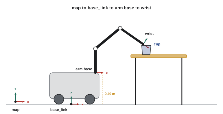
Real systems add layers: the cup's position comes from a camera whose own pose is another link in the chain, the base pose comes from localization with uncertainty, and the gripper needs an orientation as well as a position. But the structure is exactly the one built in this course: frames, rotations, transforms, forward and inverse kinematics, Jacobians and an awareness of where the robot moves well. ROB-300 adds the forces and dynamics, ROB-340 the localization, and ROB-350 the motion planning that turn this geometry into a working robot.
Common mistakes
MistakeCommanding a differential-drive robot to move sideways.
InsteadIt is nonholonomic; plan paths it can follow, made of arcs and straight segments.
MistakeIntegrating odometry with the heading at the start of each step.
InsteadUse the mid-step heading or the exact arc update.
MistakeTrusting wheel odometry over long distances.
InsteadCalibrate wheel radius and track width, and fuse odometry with other sensors to correct drift.
MistakeSteering both front wheels of a car-like robot to the same angle.
InsteadAckermann geometry turns the inner wheel more sharply so all wheels share one ICR.
MistakeChoosing a mobile manipulator's stopping point without considering reach and manipulability.
InsteadPick the base pose so targets lie near 70 to 80 % of arm reach and away from singularities.
Summary and key terms
- A wheeled robot's pose is in SE(2); body velocities are rotated by the heading into world velocities.
- Differential drive: \( v = r(\omega_R + \omega_L)/2 \) and \( \omega = r(\omega_R - \omega_L)/b \), turning about an ICR.
- Rolling without slipping gives nonholonomic constraints: no sideways motion, though every pose remains reachable.
- Odometry integrates wheel motion into pose and drifts, so it is fused with other sensors.
- Car-like robots follow the bicycle model with a minimum turning radius and Ackermann wheel angles.
- Mecanum and omni wheels give holonomic motion with three instantaneous degrees of freedom.
- Mobile manipulators chain a base pose with arm kinematics, and base placement is part of solving the task.
- Differential drive
- A base with two independently driven wheels on a common axle.
- Track width
- The distance between the left and right wheels.
- Instantaneous center of rotation
- The point about which a body is rotating at a given instant.
- Unicycle model
- A simplified model with forward speed and turn rate as inputs.
- Nonholonomic constraint
- A constraint on velocities that cannot be integrated into one on positions.
- Odometry
- Estimating pose by integrating wheel motion over time.
- Ackermann steering
- A steering geometry that turns the inner wheel more than the outer so all wheels share one ICR.
- Bicycle model
- A car-like vehicle model with one steered front wheel and one rear wheel.
- Mecanum wheel
- A wheel with rollers at 45° that allows omnidirectional motion.
- Mobile manipulator
- A robot arm mounted on a mobile base.
Practice problems
Work each problem on paper first, then reveal the answer to check.
A differential-drive robot has r = 0.1 m and both wheels at 5 rad/s. What is its speed?
Show answer
0.5 m/s straight ahead.
Same robot, b = 0.5 m, wheels at +5 and −5 rad/s. What is its turn rate?
Show answer
\( 0.1 \times 10/0.5 = 2 \) rad/s, spinning on the spot.
What is the turn radius for v = 0.6 m/s and ω = 0.3 rad/s?
Show answer
2 m.
Find the wheel speeds for v = 0.5 m/s, ω = 0 with r = 0.05 m.
Show answer
10 rad/s each.
Write the rolling constraint of a differential-drive robot.
Show answer
\( \dot{x}\sin\theta - \dot{y}\cos\theta = 0 \).
An encoder gives 2,000 counts per revolution on a 0.08 m radius wheel. What distance is one count?
Show answer
\( 2\pi \times 0.08/2000 \approx 0.25 \) mm.
A car has wheelbase 2.7 m and maximum steering angle 35°. What is its minimum turning radius at the rear axle?
Show answer
\( 2.7/\tan 35^\circ \approx 3.9 \) m.
How many instantaneous DOF does a mecanum platform have?
Show answer
Three.
Why is the mecanum forward kinematics computed with a pseudoinverse?
Show answer
Four wheel speeds over-determine three body velocities.
A target is 0.2 m from an arm with 0.75 m reach. Should the base move closer or further away?
Show answer
Further away, to put the target nearer 70 to 80 % of reach.
Lesson quiz · 5 questions
Score 60% or more to complete this lesson.
Create a free account to save your progress, take quizzes and earn a certificate.