Entanglement: Bell states, Bell inequalities and nonlocality

In 1935 Albert Einstein, Boris Podolsky and Nathan Rosen published a short paper arguing that quantum mechanics could not be a complete description of reality. Their argument used a pair of particles in an entangled state, prepared so that measuring one would reveal the result of the same measurement on the other, however far away it was. They concluded that the results must have been fixed in advance by properties the theory leaves out. For almost thirty years the question seemed philosophical. Then in 1964 John Bell, a physicist at CERN, showed that it could be settled by experiment: any theory in which results are fixed in advance by local properties must satisfy a certain inequality, and quantum mechanics predicts that it can be violated. This lesson derives Bell's result in the form most used today, the CHSH inequality, and describes the experiments that tested it.

The Bell states

Two qubits have a four-dimensional state space. A convenient basis consists of the four Bell states,

Each is maximally entangled: the reduced state of either qubit is \(1/2\), with one bit of entanglement entropy. The singlet \(|\Psi^-\rangle\) is special because it is rotationally invariant. For any direction \(\hat{\mathbf n}\) it has the same form, \((|{\uparrow_n}{\downarrow_n}\rangle - |{\downarrow_n}{\uparrow_n}\rangle)/\sqrt2\), so measurements of the two spins along any common axis always give opposite results. For measurements along different axes \(\hat{\mathbf a}\) and \(\hat{\mathbf b}\), the correlation is

Here \(E\) is the average of the product of the two \(\pm1\) results. Each result alone is completely random, with equal chances of \(+1\) and \(-1\) for any axis, because the reduced states are maximally mixed. All the structure is in the correlation.

Local hidden variables

EPR's view can be made precise. Suppose each pair carries some hidden variable \(\lambda\), distributed with probability density \(\rho(\lambda)\), that fixes the results in advance. Locality means that the result on side A depends only on the setting \(a\) chosen there and on \(\lambda\), not on the distant setting \(b\): \(A(a, \lambda) = \pm1\) and \(B(b, \lambda) = \pm1\). Then

Such models can reproduce some quantum predictions easily. Perfect anticorrelation for equal settings is obtained by letting \(\lambda\) be a direction and setting \(A = \operatorname{sign}(\hat{\mathbf a}\cdot\boldsymbol\lambda)\) and \(B = -\operatorname{sign}(\hat{\mathbf b}\cdot\boldsymbol\lambda)\). The question Bell asked was whether any such model can reproduce all of them.

The CHSH inequality

In 1969 John Clauser, Michael Horne, Abner Shimony and Richard Holt derived a version of Bell's inequality suited to real experiments. Let each side choose between two settings, \(a\) or \(a'\) and \(b\) or \(b'\). For a fixed \(\lambda\), write \(A = A(a, \lambda)\), \(A' = A(a', \lambda)\) and similarly \(B\), \(B'\). Then

because \(B\) and \(B'\) are each \(\pm1\), so one of \(B - B'\) and \(B + B'\) is zero and the other is \(\pm2\). Averaging over \(\lambda\) gives the CHSH inequality:

The derivation used only three assumptions: that results are determined by \(\lambda\) and the local setting, that the distribution of \(\lambda\) does not depend on the settings, and that the outcomes are \(\pm1\). It does not assume anything about quantum mechanics, and it holds for stochastic models too, since randomness can always be absorbed into \(\lambda\).

Quantum mechanics violates it. With the singlet correlation \(E = -\cos(\theta_a - \theta_b)\) and the settings \(a = 0\), \(a' = \pi/2\), \(b = \pi/4\), \(b' = 3\pi/4\) in one plane,

Boris Tsirelson proved in 1980 that \(2\sqrt2\) is the largest value quantum mechanics allows. The proof is short: with \(\mathcal B = A \otimes (B - B') + A' \otimes (B + B')\) for observables with eigenvalues \(\pm1\), one finds \(\mathcal B^2 = 4 + [A, A'] \otimes [B, B']\), and each commutator has norm at most 2, so \(\|\mathcal B\| \le 2\sqrt2\). Quantum mechanics is therefore nonlocal, but in a limited way. Theories with even stronger correlations, such as the hypothetical Popescu–Rohrlich box with \(|S| = 4\), are consistent with relativity but not realized in nature, as far as anyone knows.

import math, random

# Quantum prediction for the singlet: E(a, b) = -cos(a - b) for measurement angles a, b in one plane
def E_q(a, b): return -math.cos(a - b)
a, ap, b, bp = 0.0, math.pi / 2, math.pi / 4, 3 * math.pi / 4
S_q = E_q(a, b) - E_q(a, bp) + E_q(ap, b) + E_q(ap, bp)
print(f"Quantum CHSH value with the optimal angles: |S| = {abs(S_q):.5f}  (Tsirelson bound 2 sqrt 2 = {2 * math.sqrt(2):.5f})")

# Local hidden variables: each pair carries an angle lam; each side's outcome is a fixed function of (setting, lam)
# ('sign' averages over evenly spaced lam; 'random' draws outcomes by chance)
random.seed(1964)
def lhv(model, x, lam):
    if model == "sign": return 1 if math.cos(x - lam) >= 0 else -1          # classic deterministic model
    if model == "random": return random.choice((1, -1))                      # no correlation at all
def E_lhv(model, x, y, N=200000):
    tot = 0
    for i in range(N):
        lam = 2 * math.pi * (i + 0.5) / N if model == 'sign' else random.uniform(0, 2 * math.pi)
        tot += lhv(model, x, lam) * -lhv(model, y, lam)                         # anticorrelated like the singlet
    return tot / N
for model in ("sign", "random"):
    S = E_lhv(model, a, b) - E_lhv(model, a, bp) + E_lhv(model, ap, b) + E_lhv(model, ap, bp)
    print(f"Local model '{model}': |S| = {abs(S):.3f}  (any local model satisfies |S| <= 2)")
print()

# The best a local deterministic strategy can do: enumerate all 16 assignments of +/-1 to A, A', B, B'
best = max(abs(A * B - A * Bp + Ap * B + Ap * Bp) for A in (1, -1) for Ap in (1, -1) for B in (1, -1) for Bp in (1, -1))
print(f"Maximum of |AB - AB' + A'B + A'B'| over all 16 deterministic assignments = {best}")
print()

# Correlation curves: quantum -cos(theta) vs the 'sign' model, which is linear in theta
print(" angle (deg)   quantum E    local 'sign' model E")
for deg in (0, 22.5, 45, 67.5, 90, 135, 180):
    th = math.radians(deg)
    print(f"   {deg:6.1f}      {E_q(0, th) + 0.0 if abs(E_q(0, th)) > 1e-12 else 0.0:+.4f}      {E_lhv('sign', 0, th, 100000) + 0.0:+.4f}  (exact {-1 + 2 * th / math.pi:+.4f})")
print()

# Werner states: rho = p |singlet><singlet| + (1 - p) I/4 violate CHSH only when p > 1/sqrt2
print("Werner state mixing p:   max CHSH = 2 sqrt2 p   violates?  entangled (p > 1/3)?")
for p in (0.3, 0.5, 0.7, 0.75, 0.9):
    print(f"        {p:4.2f}               {2 * math.sqrt(2) * p:.3f}          {'yes' if 2 * math.sqrt(2) * p > 2 else 'no '}        {'yes' if p > 1 / 3 else 'no'}")

Quantum CHSH value with the optimal angles: |S| = 2.82843  (Tsirelson bound 2 sqrt 2 = 2.82843)
Local model 'sign': |S| = 2.000  (any local model satisfies |S| <= 2)
Local model 'random': |S| = 0.004  (any local model satisfies |S| <= 2)

Maximum of |AB - AB' + A'B + A'B'| over all 16 deterministic assignments = 2

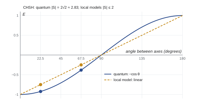
 angle (deg)   quantum E    local 'sign' model E
      0.0      -1.0000      -1.0000  (exact -1.0000)
     22.5      -0.9239      -0.7500  (exact -0.7500)
     45.0      -0.7071      -0.5000  (exact -0.5000)
     67.5      -0.3827      -0.2500  (exact -0.2500)
     90.0      +0.0000      +0.0000  (exact +0.0000)
    135.0      +0.7071      +0.5000  (exact +0.5000)
    180.0      +1.0000      +1.0000  (exact +1.0000)

Werner state mixing p:   max CHSH = 2 sqrt2 p   violates?  entangled (p > 1/3)?
        0.30               0.849          no         no
        0.50               1.414          no         yes
        0.70               1.980          no         yes
        0.75               2.121          yes        yes
        0.90               2.546          yes        yes

The program confirms the three key numbers. The quantum CHSH value at the optimal angles equals the Tsirelson bound. The local "sign" model, in which each particle carries a random direction and each detector reports the sign of its projection, reaches exactly 2, the most a local model can do; a model with uncorrelated random outcomes gives 0. Enumerating all 16 deterministic assignments of \(\pm1\) to \(A, A', B, B'\) shows that \(|S|\) never exceeds 2. The correlation curves show why: the local model's correlation is linear in the angle, while the quantum one follows a cosine, which bends further from zero at intermediate angles.

Mixed states and the limits of violation

Real sources do not produce perfect singlets. A useful model is the Werner state, \(\rho = p|\Psi^-\rangle\langle\Psi^-| + (1 - p)\,1/4\), a singlet mixed with white noise. Its correlations are those of the singlet multiplied by \(p\), so the maximum CHSH value is \(2\sqrt2p\), and a violation requires \(p > 1/\sqrt2 \approx 0.71\). Yet the state is entangled, in the sense that it cannot be written as a mixture of product states, for every \(p > 1/3\). Reinhard Werner showed in 1989 that some entangled states admit local hidden-variable models for all projective measurements. Entanglement and Bell nonlocality are therefore related but different: every state that violates a Bell inequality is entangled, but not every entangled state violates one. Deciding whether a mixed state is entangled is hard in general; for two qubits, the Peres–Horodecki criterion of 1996, the partial transpose test, decides it exactly.

The experiments

The first tests, by Stuart Freedman and John Clauser at Berkeley in 1972, used pairs of photons emitted in a cascade of calcium atoms and found correlations in agreement with quantum mechanics and in violation of Bell's inequality. Alain Aspect and colleagues at Orsay in 1981 and 1982 improved the method and, in the last experiment of the series, switched the analyzer settings while the photons were in flight, so that no signal traveling at light speed could carry one setting to the other side in time. Later experiments used entangled photons from nonlinear crystals and separated the detectors by kilometers; in 1998 Anton Zeilinger's group in Innsbruck chose the settings with fast random-number generators.

Two loopholes remained. The locality loophole requires the setting choices and measurements to be spacelike separated. The detection loophole arises because photon detectors miss many photons; if the detected pairs are an unfair sample, a local model can mimic the violation. In 2015 three experiments closed both at once. Ronald Hanson's group at Delft entangled electron spins in diamond 1.3 km apart and found \(S = 2.42 \pm 0.20\). Groups led by Zeilinger in Vienna and by Lynden Shalm and colleagues at NIST in Boulder used highly efficient photon detectors. All three rejected local realism, and the 2022 Nobel Prize went to Aspect, Clauser and Zeilinger. A 2018 experiment, the Big Bell Test, even used choices made by about 100,000 volunteers playing an online game to set the detectors.

What does a violation mean? It rules out every theory that is both local and realistic in Bell's sense. It does not allow signals faster than light: Alice's results are random whatever Bob does, and the correlation shows up only when the two records are brought together by ordinary means. This no-signaling property follows from the fact that Bob's operations do not change Alice's reduced density matrix. Quantum mechanics is consistent with relativity, but it cannot be replaced by any local account in which measurement results exist before they are measured.

Entanglement as a resource

Since the 1990s entanglement has been treated as a resource, like energy, that can be created, transferred and consumed. A shared Bell pair plus two classical bits lets one party teleport an unknown qubit to the other (lesson 10). A shared Bell pair plus one qubit sent lets two classical bits be transmitted, superdense coding. Entanglement certified by a Bell violation guarantees that the measurement results are random even to someone who built the devices, the basis of device-independent random-number generation and of the entanglement-based key distribution proposed by Artur Ekert in 1991. Pairs whose entanglement has been degraded by noise can be distilled into fewer, purer pairs, which is how quantum repeaters are designed to carry entanglement over long fibers.