Time-dependent perturbation theory revisited: the Dyson series, harmonic perturbations and the adiabatic theorem

PHYS-373 introduced time-dependent perturbation theory to first order and used it for Rabi oscillations, Fermi's golden rule and selection rules. That is enough for most spectroscopy, but it leaves open questions. What is the second-order correction, and when is it needed? What happens when a Hamiltonian changes slowly rather than weakly? And why does a quantum state taken slowly around a closed loop return with a phase that depends only on the geometry of the loop? This lesson answers all three. The tool for the first is the Dyson series, the formal solution of the interaction-picture equation from lesson 2. The tools for the others are the adiabatic theorem and Berry's geometric phase.

The Dyson series

In the interaction picture the time-evolution operator \(U_I(t, t_0)\) obeys \(i\hbar\,\partial_tU_I = V_I(t)U_I\) with \(U_I(t_0, t_0) = 1\). Integrating once turns this into an integral equation,

which can be solved by iteration: substitute the right-hand side into itself again and again. The result is the Dyson series, published by Freeman Dyson in 1949 in his work on quantum electrodynamics:

The times are ordered, \(t \ge t_1 \ge t_2 \ge \cdots \ge t_n \ge t_0\), and the operators are written with later times to the left. Each term has a physical reading. The system evolves freely, is kicked by the perturbation at time \(t_n\), evolves freely again, is kicked at \(t_{n-1}\), and so on, and the amplitude sums over all orders and all times of the kicks. Feynman diagrams are a pictorial bookkeeping of exactly these terms.

Because the integrand is ordered, the series can be written compactly with the time-ordering operator \(\mathcal T\), which rearranges a product so that later times stand to the left. Then the region of integration can be extended to a full cube, at the cost of a factor \(1/n!\) that cancels the \(n!\) orderings:

If the \(V_I\) at different times commuted, \(\mathcal T\) would do nothing and this would be an ordinary exponential. In general they do not, and the time ordering carries all the difficulty.

Taking matrix elements between eigenstates of \(H_0\) gives the familiar amplitudes. Starting in state \(i\), the amplitude to be found in \(f\) is

The second-order term describes transitions through an intermediate state \(m\). It matters when the direct matrix element \(V_{fi}\) vanishes, for instance because of a selection rule, while \(V_{fm}\) and \(V_{mi}\) do not. Two-photon absorption, Raman scattering and the two-photon decay of hydrogen \(2s\) are second-order processes of this kind. The second-order term for \(c_i\) itself, the amplitude to remain, accounts for the loss of probability to other states at the same order as \(|c_f|^2\), which keeps the total probability equal to one through second order.

A pulse and the limits of perturbation theory

The program applies the series to a two-level system with splitting \(\omega\), driven by a Gaussian pulse \(V(t) = g\,e^{-t^2/\tau^2}\). The first-order amplitude can be done analytically,

in units with \(\hbar = 1\). The Gaussian factor shows a general rule: the transition probability depends on the Fourier component of the perturbation at the transition frequency. A pulse much longer than \(1/\omega\) has almost no such component and causes almost no transitions. This is the adiabatic limit, discussed below. A short pulse has a broad spectrum and can cause transitions even far from resonance.

Harmonic perturbations and energy conservation

For a perturbation \(V(t) = Fe^{-i\omega t} + F^\dagger e^{i\omega t}\) switched on at \(t = 0\), the first-order amplitude contains the two denominators \(\omega_{fi} - \omega\) and \(\omega_{fi} + \omega\). The first resonance is absorption, \(E_f = E_i + \hbar\omega\); the second is stimulated emission, \(E_f = E_i - \hbar\omega\). As \(t\) grows the resonant factor sharpens into the function \((2\pi/\hbar)t\,\delta(E_f - E_i \mp \hbar\omega)\), giving the golden rule of PHYS-373: energy is conserved in the long-time limit, but only to within \(\hbar/t\) for a finite time. At second order, energy need not be conserved in the intermediate state. The system can pass through a virtual state \(m\) with \(E_m \ne E_i + \hbar\omega\), with an amplitude suppressed by the energy denominator \(E_m - E_i - \hbar\omega\). This is the sense in which perturbation theory allows virtual transitions that violate energy conservation for a short time.

The adiabatic theorem

Now suppose \(H(t)\) changes slowly but not necessarily by a small amount, such as a magnetic field that rotates, or the separation of two nuclei in a molecule as they collide. Let \(|n(t)\rangle\) be the instantaneous eigenstates, \(H(t)|n(t)\rangle = E_n(t)|n(t)\rangle\). The adiabatic theorem, proved by Max Born and Vladimir Fock in 1928, states that a system that starts in \(|n(0)\rangle\) stays in \(|n(t)\rangle\), apart from a phase, provided that the level \(E_n\) remains non-degenerate and the change is slow compared with the time scale set by the gap to other levels.

To see why, expand \(|\psi(t)\rangle = \sum_mc_m(t)e^{i\theta_m(t)}|m(t)\rangle\) with the dynamical phase \(\theta_m = -(1/\hbar)\int_0^tE_m\,dt'\). Substituting into the Schrödinger equation gives

The terms that mix levels are proportional to the rate of change \(\dot H\) and inversely proportional to the energy gap, and they oscillate rapidly through the phase factor. When \(|\langle m|\dot H|n\rangle| \ll (E_n - E_m)^2/\hbar\), the mixing averages away and each \(c_m\) evolves on its own. The adiabatic condition is therefore a comparison between the rate of change and the square of the gap.

Landau–Zener transitions

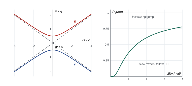
The simplest test of the adiabatic theorem is an avoided crossing. Two diabatic states, such as two spin states in a field that is swept through zero, have energies \(\pm vt/2\) that cross at \(t = 0\). A coupling \(\Delta/2\) between them turns the crossing into an avoided crossing with minimum gap \(\Delta\):

If the sweep is slow the system follows the lower adiabatic level and ends in the other diabatic state. If it is fast it jumps across the gap and stays in its original diabatic state. Lev Landau and Clarence Zener found the exact probability of the jump in 1932, independently, as did Ernst Stueckelberg and Ettore Majorana:

The exponent compares the square of the gap with the sweep rate, as the adiabatic condition predicted. Landau–Zener physics governs electron transfer in chemical reactions, the behavior of neutrinos crossing the dense interior of the Sun (the MSW effect), and adiabatic quantum computing, in which a hard problem is encoded in the ground state of a Hamiltonian reached by a slow sweep.

Berry's geometric phase

In the adiabatic limit a state picks up the dynamical phase \(\theta_n\), which depends on how long the process takes. In 1984 Michael Berry pointed out that it also picks up a second phase that does not. Substituting \(c_n = e^{i\gamma_n}\) into the adiabatic equation above, with the mixing terms dropped, gives \(\dot\gamma_n = i\langle n|\dot n\rangle\). If the Hamiltonian depends on parameters \(\mathbf R\) taken around a closed loop \(C\), the accumulated phase is

This depends only on the path in parameter space, not on the speed, so it is called geometric. It cannot be removed by redefining the phases of the eigenstates, because any such redefinition must be single-valued around the loop, and for a closed loop \(\gamma_n\) is gauge invariant. The integrand acts like a vector potential in parameter space, and by Stokes's theorem \(\gamma_n\) is the flux of the corresponding curvature through the loop.

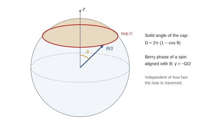
For a spin one-half aligned with a magnetic field whose direction traces a loop on the sphere, the result is particularly simple:

where \(\Omega\) is the solid angle the loop subtends at the center of the sphere. For a spin \(s\) state with \(m_s = m\), the phase is \(-m\Omega\). The curvature is that of a magnetic monopole at the origin of parameter space, located where the two levels become degenerate. Berry phases have been measured with neutrons in rotating fields and with light in coiled optical fibers, where the polarization rotates by an amount set by the geometry of the coil. Related geometric phases explain the Aharonov–Bohm effect, the quantization of the Hall conductance in topological materials, and geometric quantum gates.

import cmath, math

def rk4(f, y, t0, t1, n):
    h = (t1 - t0) / n; t = t0
    for _ in range(n):
        k1 = f(t, y); k2 = f(t + h / 2, [a + h / 2 * b for a, b in zip(y, k1)])
        k3 = f(t + h / 2, [a + h / 2 * b for a, b in zip(y, k2)]); k4 = f(t + h, [a + h * b for a, b in zip(y, k3)])
        y = [a + h / 6 * (p + 2 * q + 2 * r + s) for a, p, q, r, s in zip(y, k1, k2, k3, k4)]; t += h
    return y

# 1. Dyson series: two levels split by w, Gaussian pulse V(t) = g exp(-(t/tau)^2) coupling them (hbar = 1)
w, tau, T = 1.0, 2.0, 12.0
def exact(g):
    V = lambda t: g * math.exp(-(t / tau) ** 2)
    f = lambda t, c: [-1j * V(t) * cmath.exp(-1j * w * t) * c[1], -1j * V(t) * cmath.exp(1j * w * t) * c[0]]
    return rk4(f, [1 + 0j, 0j], -T, T, 6000)
def dyson(g, n=6000):
    h = 2 * T / n; c1 = 0j; c2 = 0j; inner = 0j
    for k in range(n):
        t = -T + (k + 0.5) * h; V = g * math.exp(-(t / tau) ** 2)
        c2 += -V * cmath.exp(-1j * w * t) * inner * h      # second-order term for c_a
        inner += V * cmath.exp(1j * w * t) * h
        c1 += -1j * V * cmath.exp(1j * w * t) * h            # first-order term for c_b
    return 1 + c2, c1
print("Gaussian pulse: exact vs Dyson series (first order for c_b, second order for c_a)")
print("   g     P_b exact   P_b 1st order   |c_a|^2 exact   |c_a|^2 to 2nd order")
for g in (0.05, 0.2, 0.5):
    ca, cb = exact(g); da, db = dyson(g)
    print(f"  {g:4.2f}   {abs(cb) ** 2:.6f}     {abs(db) ** 2:.6f}        {abs(ca) ** 2:.6f}        {abs(da) ** 2:.6f}")
print(f"  analytic first order at g = 0.05: {(0.05 * tau * math.sqrt(math.pi) * math.exp(-w * w * tau * tau / 4)) ** 2:.6f}")
print()

# 2. Landau-Zener: H = (v t/2) sz + (D/2) sx swept from -T to +T
def adiabatic(t, D, v, upper):
    """Normalized eigenvector of H(t) = (v t/2) sz + (D/2) sx; upper or lower energy."""
    E = math.hypot(v * t, D) / 2 * (1 if upper else -1)
    a, b = D / 2, E - v * t / 2                        # (H - E) x = 0  gives  x = (D/2, E - v t/2)
    n = math.hypot(a, b); return [a / n, b / n]
def lz(D, v, T=40.0):
    n = int(20 * v * T * T) + 1000
    f = lambda t, c: [-1j * (v * t / 2 * c[0] + D / 2 * c[1]), -1j * (D / 2 * c[0] - v * t / 2 * c[1])]
    c = rk4(f, [complex(x) for x in adiabatic(-T, D, v, False)], -T, T, n)   # start in the lower level
    up = adiabatic(T, D, v, True)
    return abs(up[0] * c[0] + up[1] * c[1]) ** 2         # jumped to the upper level = stayed diabatic
print("Landau-Zener sweep: probability of a diabatic jump (ending in the upper level)")
print("   D     v     numeric    exp(-pi D^2 / 2v)")
for D, v in ((0.5, 1.0), (1.0, 1.0), (1.0, 4.0)):
    print(f"  {D:4.2f}  {v:4.1f}   {lz(D, v):.4f}     {math.exp(-math.pi * D * D / (2 * v)):.4f}")
print()

# 3. Berry phase: spin one-half aligned with a field whose direction circles at polar angle theta
def berry(theta, N=2000):
    st = lambda ph: (math.cos(theta / 2), cmath.exp(1j * ph) * math.sin(theta / 2))
    prod = 1 + 0j
    for k in range(N):
        a = st(2 * math.pi * k / N); b = st(2 * math.pi * (k + 1) / N)
        prod *= a[0].conjugate() * b[0] + a[1].conjugate() * b[1]
    return -cmath.phase(prod)
print("Berry phase for a field direction looping at polar angle theta")
print("   theta (deg)   numeric     -pi(1 - cos theta)   solid angle / 4pi")
for deg in (30, 60, 90, 120):
    th = math.radians(deg); g = berry(th); ex = -math.pi * (1 - math.cos(th))
    ex_w = (ex + math.pi) % (2 * math.pi) - math.pi
    print(f"     {deg:4d}       {g:+.5f}       {ex_w:+.5f}           {(1 - math.cos(th)) / 2:.4f}")

Gaussian pulse: exact vs Dyson series (first order for c_b, second order for c_a)
   g     P_b exact   P_b 1st order   |c_a|^2 exact   |c_a|^2 to 2nd order
  0.05   0.004196     0.004252        0.995804        0.995842
  0.20   0.054857     0.068027        0.945143        0.949988
  0.50   0.086122     0.425168        0.913878        1.265372
  analytic first order at g = 0.05: 0.004252

Landau-Zener sweep: probability of a diabatic jump (ending in the upper level)
   D     v     numeric    exp(-pi D^2 / 2v)
  0.50   1.0   0.6752     0.6752
  1.00   1.0   0.2079     0.2079
  1.00   4.0   0.6752     0.6752

Berry phase for a field direction looping at polar angle theta
   theta (deg)   numeric     -pi(1 - cos theta)   solid angle / 4pi
       30       -0.42089       -0.42089           0.0670
       60       -1.57080       -1.57080           0.2500
       90       -3.14159       -3.14159           0.5000
      120       +1.57080       +1.57080           0.7500

Three lessons come from the output. For a weak pulse, \(g = 0.05\), first order gives the transition probability to within about one part in a hundred, and the analytic Gaussian formula matches the numerical first-order integral. At \(g = 0.5\) perturbation theory fails badly. The first-order probability is five times the exact one, and the second-order expression for \(|c_a|^2\) even exceeds 1, because a truncated series need not respect the normalization that the full series preserves. For the Landau–Zener sweep, the program starts in the lower adiabatic level well before the crossing and projects onto the upper level well after it; the result reproduces the exact exponential to four places. The first and third cases have the same value of \(\Delta^2/v\) and so the same jump probability, showing that only this combination matters. The Berry phase is computed as the phase of the product of overlaps of neighboring states around the loop, a discrete version of the integral that is gauge invariant. It agrees with \(-\pi(1 - \cos\theta)\) when reduced to the interval from \(-\pi\) to \(\pi\).