Resonances, bound states and low-energy scattering

At low energy, scattering becomes simple in one way and subtle in another. It is simple because only the s-wave, \(\ell = 0\), reaches the target: a particle with angular momentum \(\ell\hbar\) and momentum \(\hbar k\) passes at a distance of about \(\ell/k\), which for small \(k\) is far outside a short-range potential. The whole effect of the potential then reduces to a single length, the scattering length \(a\). It is subtle because \(a\) can be large, of either sign, and very sensitive to the potential near the threshold for a bound state. This lesson connects low-energy scattering to bound states, explains resonances as nearly bound states, and ends with the Feshbach resonances that let experimenters tune \(a\) in ultracold atomic gases simply by changing a magnetic field.

The scattering length

For \(\ell = 0\) the radial function \(u(r) = r\psi\) outside a potential of range \(R\) is \(u \propto \sin(kr + \delta_0)\). As \(k \to 0\), the phase shift behaves as \(\delta_0 \to -ka\) (modulo \(\pi\)), which defines the scattering length \(a\). At zero energy the exterior solution becomes a straight line, \(u \propto (r - a)\), and \(a\) is simply where that line, extended inward, crosses zero. The amplitude and cross-section at low energy are

For a hard sphere of radius \(R\), \(a = R\) and \(\sigma = 4\pi R^2\), four times the geometric cross-section, a purely wave effect. For an attractive square well of depth \(V_0\), matching the interior solution \(\sin Kr\) with \(K = \sqrt{2mV_0}/\hbar\) to the exterior line gives

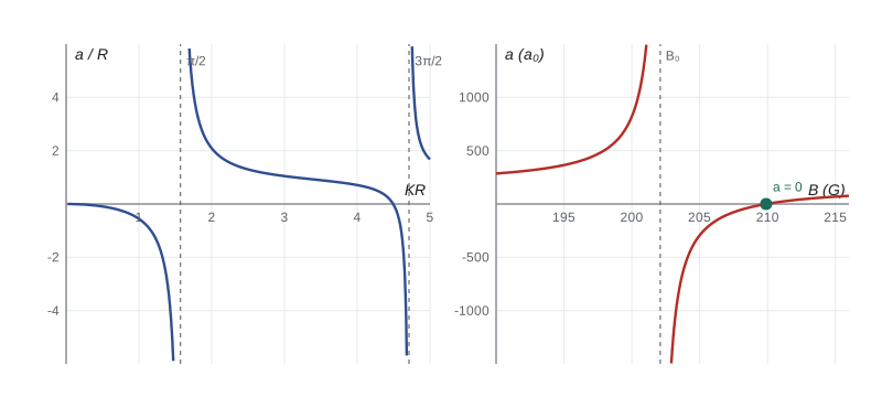
For a shallow well \(a\) is small and negative, meaning the line crosses zero outside the well on the far side; the interaction is weakly attractive. As the well deepens, \(KR \to \pi/2\), \(\tan KR\) diverges and \(a \to -\infty\). Just beyond \(\pi/2\) a bound state appears and \(a\) jumps to \(+\infty\), then decreases. The pattern repeats at \(KR = 3\pi/2, 5\pi/2, \ldots\), each time a new bound state appears. So a large scattering length signals a bound state, real or virtual, very close to zero energy. In that case the cross-section \(4\pi a^2\) can be enormous compared with the size of the potential.

Shallow bound states and universality

When \(a\) is large and positive there is a shallow bound state. Outside the potential its wave function is \(u \propto e^{-\kappa r}\), with binding energy \(E_b = \hbar^2\kappa^2/2m\). Matching at low energy requires \(\kappa \approx 1/a\), so

The bound state is far larger than the potential that holds it, and its properties depend on \(a\) alone, not on the details of the potential. This is called universality. The deuteron is a natural example: the neutron–proton scattering length in the spin-triplet state is about 5.4 fm, compared with a nuclear force range of about 1.4 fm, and the deuteron binding energy of 2.22 MeV is close to the universal estimate once the finite range is included. The next correction comes from the effective-range expansion,

which adds a second parameter, the effective range \(r_e\), of order the size of the potential. With it the bound-state condition becomes \(\kappa = 1/a + r_e\kappa^2/2\), which to the same order gives \(E_b \approx \hbar^2/2m(a - r_e/2)^2\). The program tests both formulas. With \(r_e \approx R\) the second one tracks the exact binding energy closely until the bound state is no longer shallow.

Resonances

A different kind of large effect occurs when a potential has a barrier that can trap a particle temporarily. For \(\ell \ge 1\) the centrifugal term \(\ell(\ell + 1)\hbar^2/2mr^2\) provides such a barrier around an attractive well. If the well is almost, but not quite, deep enough to bind a state, there is a quasi-bound state at a small positive energy \(E_r\). A particle with energy near \(E_r\) can tunnel in, stay for a time, and tunnel out. The phase shift rises rapidly through \(\pi/2\) at \(E_r\) and the partial cross-section reaches its maximum allowed value, \(4\pi(2\ell + 1)/k^2\). Near the resonance,

This is the Breit–Wigner formula, introduced by Gregory Breit and Eugene Wigner in 1936 for neutron capture by nuclei. The width \(\Gamma\) is related to the lifetime of the quasi-bound state by \(\tau = \hbar/\Gamma\), and the time delay of the scattered wave, \(2\hbar\,d\delta/dE\), equals \(4\hbar/\Gamma\) at the peak. In the complex energy plane a resonance is a pole of the amplitude at \(E = E_r - i\Gamma/2\), just below the real axis, while a bound state is a pole on the negative real axis. As the well deepens, the resonance pole moves toward zero energy and becomes a bound state. The same mathematics describes resonances in particle physics, such as the \(Z\) boson with \(\Gamma \approx 2.5\) GeV, nuclear resonances in neutron cross-sections, and atomic autoionizing states.

import math
# Units hbar^2/2m = 1 (E = k^2), attractive square well of depth V0 and radius R = 1.

def scat_length(V0, R=1.0):
    K = math.sqrt(V0); return R - math.tan(K * R) / K

print("Scattering length of a square well as it is deepened (bound states appear at sqrt(V0) R = pi/2, 3pi/2)")
print("  sqrt(V0)R    a/R")
for g in (0.5, 1.0, 1.4, 1.5, 1.55, 1.6, 1.7, 2.0, 3.0, 4.6, 4.8):
    print(f"   {g:5.2f}   {scat_length(g * g):+9.3f}")
print()

# Shallow bound state: binding energy vs the universal estimate E_b = 1/a^2 (units hbar^2/2m)
def bound_energy(V0, R=1.0):
    """Lowest s-wave bound state: solve K cot(K R) = -kappa with K^2 + kappa^2 = V0, by bisection."""
    f = lambda kap: math.sqrt(V0 - kap * kap) / math.tan(math.sqrt(V0 - kap * kap) * R) + kap
    lo, hi = 1e-9, math.sqrt(V0) - 1e-9
    for _ in range(200):
        mid = (lo + hi) / 2
        if f(lo) * f(mid) <= 0: hi = mid
        else: lo = mid
    return mid * mid
print("Shallow bound state near threshold: E_b compared with 1/a^2")
print("  sqrt(V0)R     a/R      E_b       1/a^2     1/(a - r_e/2)^2 with r_e = R")
for g in (1.60, 1.65, 1.75, 2.0):
    V0 = g * g; a = scat_length(V0); Eb = bound_energy(V0)
    print(f"    {g:4.2f}    {a:7.3f}   {Eb:.5f}   {1 / a ** 2:.5f}    {1 / (a - 0.5) ** 2:.5f}")
print()

# A p-wave shape resonance just below the depth that binds a p state (sqrt(V0) R = pi)
def j0(x): return math.sin(x) / x
def j1(x): return math.sin(x) / x ** 2 - math.cos(x) / x
def n1(x): return -math.cos(x) / x ** 2 - math.sin(x) / x
def d(f, x, h=1e-6): return (f(x + h) - f(x - h)) / (2 * h)
def delta1(E, V0, R=1.0):
    k = math.sqrt(E); K = math.sqrt(E + V0)
    num = k * d(j1, k * R) * j1(K * R) - K * j1(k * R) * d(j1, K * R)
    den = k * d(n1, k * R) * j1(K * R) - K * n1(k * R) * d(j1, K * R)
    return math.atan2(num, den) % math.pi
V0 = 9.0
Es = [0.01 * i for i in range(1, 400)]
ds = [delta1(E, V0) for E in Es]
i = min(range(len(ds) - 1), key=lambda i: abs(ds[i] - math.pi / 2))
Er = Es[i]; slope = (ds[i + 1] - ds[i - 1]) / (Es[i + 1] - Es[i - 1])
print(f"p-wave resonance for V0 = {V0} (pi^2 = {math.pi ** 2:.3f} would bind it):")
print(f"  delta_1 passes pi/2 at E_r = {Er:.2f};  width Gamma = 2/(d delta/dE) = {2 / slope:.3f}")
for E in (0.2, 0.6, Er, 1.4, 2.5):
    print(f"   E = {E:4.2f}: delta_1 = {delta1(E, V0):.3f} rad, sin^2 delta_1 = {math.sin(delta1(E, V0)) ** 2:.3f}")
print()

# Feshbach resonance in a cold gas (approximate parameters for potassium-40 near 202 G)
a_bg, B0, Dl = 174.0, 202.1, 7.8          # background scattering length (Bohr radii), centre and width (gauss)
print("Feshbach resonance a(B) = a_bg [1 - Delta/(B - B0)]  (potassium-40, approximate parameters)")
for B in (190.0, 195.0, 200.0, 201.5, 202.7, 205.0, 209.9, 215.0):
    print(f"   B = {B:6.1f} G   a = {a_bg * (1 - Dl / (B - B0)):+10.0f} a0")

Scattering length of a square well as it is deepened (bound states appear at sqrt(V0) R = pi/2, 3pi/2)
  sqrt(V0)R    a/R
    0.50      -0.093
    1.00      -0.557
    1.40      -3.141
    1.50      -8.401
    1.55     -30.018
    1.60     +22.395
    1.70      +5.527
    2.00      +2.093
    3.00      +1.048
    4.60      -0.926
    4.80      +3.372

Shallow bound state near threshold: E_b compared with 1/a^2
  sqrt(V0)R     a/R      E_b       1/a^2     1/(a - r_e/2)^2 with r_e = R
    1.60     22.395   0.00209   0.00199    0.00209
    1.65      8.636   0.01513   0.01341    0.01511
    1.75      4.155   0.07538   0.05794    0.07488
    2.00      2.093   0.40710   0.22838    0.39430

p-wave resonance for V0 = 9.0 (pi^2 = 9.870 would bind it):
  delta_1 passes pi/2 at E_r = 0.35;  width Gamma = 2/(d delta/dE) = 0.326
   E = 0.20: delta_1 = 0.429 rad, sin^2 delta_1 = 0.173
   E = 0.60: delta_1 = 2.152 rad, sin^2 delta_1 = 0.699
   E = 0.35: delta_1 = 1.574 rad, sin^2 delta_1 = 1.000
   E = 1.40: delta_1 = 2.151 rad, sin^2 delta_1 = 0.699
   E = 2.50: delta_1 = 1.967 rad, sin^2 delta_1 = 0.851

Feshbach resonance a(B) = a_bg [1 - Delta/(B - B0)]  (potassium-40, approximate parameters)
   B =  190.0 G   a =       +286 a0
   B =  195.0 G   a =       +365 a0
   B =  200.0 G   a =       +820 a0
   B =  201.5 G   a =      +2436 a0
   B =  202.7 G   a =      -2088 a0
   B =  205.0 G   a =       -294 a0
   B =  209.9 G   a =         +0 a0
   B =  215.0 G   a =        +69 a0

The table of scattering lengths shows the divergence on either side of \(KR = \pi/2\): \(a = -30R\) just below, \(+22R\) just above. Near threshold, the universal estimate \(1/a^2\) and its effective-range correction both track the exact binding energy; as the well deepens and the state becomes compact, \(1/a^2\) fails by almost a factor of two, while the effective-range formula still does well. The p-wave example uses a well slightly too shallow to bind a p state, \(2mV_0R^2/\hbar^2 = 9\) against \(\pi^2 \approx 9.87\). The phase shift passes through \(\pi/2\) at \(E_r \approx 0.35\) in units of \(\hbar^2/2mR^2\), with a width of about the same size, a broad resonance because the centrifugal barrier for \(\ell = 1\) is low. Deeper wells, closer to binding the p state, give narrower resonances at lower energy, where the particle must tunnel through more of the barrier; near threshold the width grows as \(k^3\).

Feshbach resonances in ultracold gases

In an ultracold gas of alkali atoms the collision energy is a few microkelvin or less, so only s-wave scattering matters and the whole interaction is set by \(a\). Atoms colliding in one spin configuration, the open channel, can couple to a molecular bound state of a different spin configuration, the closed channel. The two channels have different magnetic moments, so a magnetic field \(B\) shifts the closed-channel bound state relative to the threshold of the open channel. When the bound state is tuned through threshold, \(a\) diverges, exactly as in the square well:

where \(a_{\text{bg}}\) is the background scattering length, \(B_0\) the position of the resonance and \(\Delta\) its width. Herman Feshbach developed the theory for nuclear reactions in 1958 and 1962. In atomic gases the resonances were first observed in 1998, in sodium by Wolfgang Ketterle's group at MIT. Since then they have become a basic tool. With \(a\) tuned large and positive, pairs of atoms form weakly bound Feshbach molecules. With \(a\) tuned large and negative in a gas of fermions, the atoms pair across the gas and form a superfluid; Deborah Jin's group at JILA in Boulder observed this fermionic condensation in potassium-40 in 2004. Tuning \(a\) to zero, on the other side of the resonance where \(B = B_0 + \Delta\), switches the interactions off entirely, so experimenters can study an ideal gas or a strongly interacting one with the same atoms.

When \(|a|\) far exceeds the spacing between atoms, the gas reaches the unitary regime, where the cross-section reaches its maximum, \(4\pi/k^2\), and the only length left is the spacing itself. Unitary Fermi gases are studied as models for the matter in neutron star crusts, where the neutron–neutron scattering length of about \(-19\) fm is also much larger than the range of the force. Feshbach resonances also make possible the Efimov states predicted by Vitaly Efimov in 1970: a geometric series of three-body bound states that appear when two-body interactions are resonant, first observed in cesium atoms in 2006.