Open quantum systems: decoherence, the Lindblad equation and T1 and T2

No real quantum system is isolated. An atom radiates into the electromagnetic field, an electron spin in a solid feels the fluctuating nuclear spins around it, and a superconducting qubit loses energy to defects in its insulating layers. Each interaction entangles the system with its environment, and since we cannot follow the environment, the system's own state becomes mixed. This process, decoherence, is why everyday objects are never seen in superpositions, and it is the main enemy of quantum technology. This lesson describes it with the Lindblad master equation and the two characteristic times \(T_1\) and \(T_2\) that every qubit specification lists.

How entanglement with an environment destroys coherence

Let a qubit start in \(\alpha|0\rangle + \beta|1\rangle\) and let it interact with an environment E that starts in \(|e\rangle\). Suppose the interaction does not change the qubit's populations but leaves a record of them in the environment:

The reduced density matrix of the qubit is then

The populations are unchanged, but the coherences are multiplied by the overlap of the two environment states. If the environment has recorded which state the qubit is in, even partially, the overlap is less than one, and if the record is complete it is zero and the qubit is in a mixture. Nothing has happened to the qubit locally; its phase information has leaked into correlations with the environment. Because environments have enormous numbers of degrees of freedom, each of which can carry a small record, the overlap typically decays exponentially in time, and faster for systems that interact more strongly. For a dust grain in air, scattering of molecules and photons makes the superposition of two positions a micrometer apart decohere in far less than a nanosecond. Wojciech Zurek and others developed this account in the 1980s; it explains why the classical world looks classical without changing the laws of quantum mechanics.

Quantum channels and Kraus operators

The general evolution of a system in contact with an environment, over a fixed time, is obtained by joining the system to the environment, evolving the whole unitarily, and tracing out the environment. The result can always be written in the operator-sum form

The Kraus operators \(K_k\) are named after Karl Kraus, who studied them in 1971 and 1983. Two channels are basic for qubits. Amplitude damping, with \(K_0 = \operatorname{diag}(1, \sqrt{1 - \gamma})\) and \(K_1 = \sqrt\gamma\,|0\rangle\langle1|\), describes the loss of energy from \(|1\rangle\) to \(|0\rangle\) with probability \(\gamma\), as in spontaneous emission. Phase damping, with \(K_0 = \sqrt{1 - \lambda/2}\,1\) and \(K_1 = \sqrt{\lambda/2}\,\sigma_z\), randomly flips the relative phase and so shrinks the coherences without changing populations. On the Bloch ball, amplitude damping pulls every state toward the north pole \(|0\rangle\), while phase damping squeezes the ball onto the \(z\) axis.

The Lindblad master equation

If the environment forgets quickly, so that its correlation time is much shorter than the times over which the system changes, the channel for a short time \(dt\) has one Kraus operator close to the identity and others of order \(\sqrt{dt}\). Taking the limit gives a differential equation, the master equation in Lindblad form:

The first term is the unitary evolution of the von Neumann equation. Each jump operator \(L_k\) describes one way the environment acts: \(L = \sqrt{\gamma_1}\,\sigma_-\) for decay from \(|1\rangle\) to \(|0\rangle\) at rate \(\gamma_1\), or \(L = \sqrt{\gamma_\phi/2}\,\sigma_z\) for dephasing. The anticommutator term keeps the trace equal to 1. Göran Lindblad (1976) and, independently, Vittorio Gorini, Andrzej Kossakowski and George Sudarshan (1976) proved that this is the most general form of a Markovian evolution that maps density matrices to density matrices, including when the system is entangled with other systems that do not evolve. The equation is often called the GKSL equation in recognition of all four.

The Lindblad equation has a physical interpretation in terms of quantum jumps. Between jumps the state evolves under an effective non-Hermitian Hamiltonian \(H - (i\hbar/2)\sum_kL_k^\dagger L_k\), and at random times a jump \(\rho \to L_k\rho L_k^\dagger\) occurs, such as the emission of a photon that could be detected. Averaging over all the possible jump records reproduces the master equation. Single trapped ions were seen to make such jumps in 1986, by groups in Hamburg, Seattle and Boulder, when the fluorescence of an ion switched off and on as it jumped in and out of a metastable level.

T1 and T2

For a qubit with amplitude damping at rate \(\gamma_1\) and pure dephasing at rate \(\gamma_\phi\), the Lindblad equation can be solved exactly. In the frame rotating at the qubit frequency,

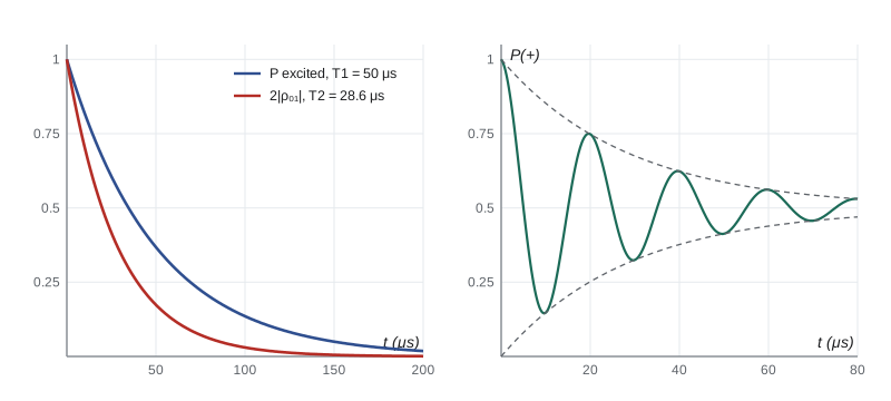
The energy relaxation time \(T_1 = 1/\gamma_1\) is the lifetime of the excited state. The coherence time \(T_2\) is the lifetime of the off-diagonal element. Energy loss also destroys coherence, but only at half the rate, because the amplitude of \(|1\rangle\) decays as \(e^{-t/2T_1}\). This gives the bound \(T_2 \le 2T_1\), reached when there is no pure dephasing. The names come from nuclear magnetic resonance: Felix Bloch's equations of 1946 for the magnetization of a sample contained a longitudinal relaxation time \(T_1\) and a transverse time \(T_2\), the same two numbers that appear in MRI contrast today.

Relaxation drives the qubit toward its thermal state. At zero temperature that is \(|0\rangle\); at temperature \(T\) the excited population settles at \(1/(e^{\hbar\omega/k_BT} + 1)\), which is why superconducting qubits at 5 GHz are operated near 20 mK in dilution refrigerators, as lesson 12 shows.

import cmath, math
# Lindblad master equation for one qubit: d rho/dt = -i[H, rho] + sum_k (L rho L^+ - (1/2){L^+ L, rho})
def mm(A, B): return [[sum(A[i][k] * B[k][j] for k in range(2)) for j in range(2)] for i in range(2)]
def dag(A): return [[A[j][i].conjugate() for j in range(2)] for i in range(2)]
def lin(A, B, a=1, b=1): return [[a * A[i][j] + b * B[i][j] for j in range(2)] for i in range(2)]

def lindblad(rho, H, Ls):
    comm = lin(mm(H, rho), mm(rho, H), -1j, 1j)
    out = comm
    for L in Ls:
        Ld = dag(L); LdL = mm(Ld, L)
        out = lin(out, mm(mm(L, rho), Ld))
        out = lin(out, lin(mm(LdL, rho), mm(rho, LdL)), 1, -0.5)
    return out

def evolve(rho, H, Ls, T, n):
    h = T / n; out = [(0.0, rho)]
    for k in range(n):
        k1 = lindblad(rho, H, Ls); k2 = lindblad(lin(rho, k1, 1, h / 2), H, Ls)
        k3 = lindblad(lin(rho, k2, 1, h / 2), H, Ls); k4 = lindblad(lin(rho, k3, 1, h), H, Ls)
        rho = [[rho[i][j] + h / 6 * (k1[i][j] + 2 * k2[i][j] + 2 * k3[i][j] + k4[i][j]) for j in range(2)] for i in range(2)]
        out.append(((k + 1) * h, rho))
    return out

gamma1, gphi = 1 / 50.0, 1 / 40.0           # rates in 1/us: T1 = 50 us; pure dephasing rate 1/40 us
sm = [[0, 1], [0, 0]]                        # lowering operator |e> -> |g>, basis order (g, e)
sz = [[1, 0], [0, -1]]
Ls = [[[math.sqrt(gamma1) * x for x in r] for r in sm], [[math.sqrt(gphi / 2) * x for x in r] for r in sz]]
H = [[0, 0], [0, 0]]                         # rotating frame on resonance

# T1: start excited, watch the population decay
traj = evolve([[0, 0], [0, 1 + 0j]], H, Ls, 200.0, 2000)
# T2: start in (|g> + |e>)/sqrt2, watch the coherence |rho_ge| decay
traj2 = evolve([[0.5 + 0j, 0.5], [0.5, 0.5]], H, Ls, 200.0, 2000)
print("  t (us)   P_excited   |rho_ge|")
for k in (0, 250, 500, 1000, 1500, 2000):
    t, r = traj[k]; _, r2 = traj2[k]
    print(f"  {t:6.1f}    {r[1][1].real:.4f}     {abs(r2[0][1]):.4f}")
def fit_rate(ts, ys):                         # least-squares slope of log y against t
    lx = [math.log(y) for y in ys]; mt = sum(ts) / len(ts); ml = sum(lx) / len(lx)
    return -sum((t - mt) * (l - ml) for t, l in zip(ts, lx)) / sum((t - mt) ** 2 for t in ts)
ts = [t for t, _ in traj[::100]]
T1 = 1 / fit_rate(ts, [r[1][1].real for _, r in traj[::100]])
T2 = 1 / fit_rate(ts, [abs(r[0][1]) for _, r in traj2[::100]])
print(f"fitted T1 = {T1:.2f} us (input 50.00),  fitted T2 = {T2:.2f} us")
print(f"prediction 1/T2 = 1/(2 T1) + gamma_phi  ->  T2 = {1 / (gamma1 / 2 + gphi):.2f} us;  limit 2 T1 = {2 / gamma1:.0f} us")
print()

# Ramsey experiment: detuning d makes the coherence precess; fringes decay with T2
d = 2 * math.pi * 0.05                      # 50 kHz detuning in rad/us
Hd = [[0, 0], [0, d]]
traj3 = evolve([[0.5 + 0j, 0.5], [0.5, 0.5]], Hd, Ls, 40.0, 400)
print("Ramsey fringes (probability of returning to |+> after free precession):")
for k in range(0, 401, 25):
    t, r = traj3[k]
    p = 0.5 + r[0][1].real                    # <+|rho|+>
    print(f"  t = {t:5.1f} us   P = {p:.3f}   " + "#" * int(40 * p))

  t (us)   P_excited   |rho_ge|
     0.0    1.0000     0.5000
    25.0    0.6065     0.2084
    50.0    0.3679     0.0869
   100.0    0.1353     0.0151
   150.0    0.0498     0.0026
   200.0    0.0183     0.0005
fitted T1 = 50.00 us (input 50.00),  fitted T2 = 28.57 us
prediction 1/T2 = 1/(2 T1) + gamma_phi  ->  T2 = 28.57 us;  limit 2 T1 = 100 us

Ramsey fringes (probability of returning to |+> after free precession):
  t =   0.0 us   P = 1.000   ########################################
  t =   2.5 us   P = 0.824   ################################
  t =   5.0 us   P = 0.500   ####################
  t =   7.5 us   P = 0.228   #########
  t =  10.0 us   P = 0.148   #####
  t =  12.5 us   P = 0.272   ##########
  t =  15.0 us   P = 0.500   ###################
  t =  17.5 us   P = 0.692   ###########################
  t =  20.0 us   P = 0.748   #############################
  t =  22.5 us   P = 0.661   ##########################
  t =  25.0 us   P = 0.500   ####################
  t =  27.5 us   P = 0.365   ##############
  t =  30.0 us   P = 0.325   #############
  t =  32.5 us   P = 0.387   ###############
  t =  35.0 us   P = 0.500   ###################
  t =  37.5 us   P = 0.595   #######################
  t =  40.0 us   P = 0.623   ########################

The program integrates the Lindblad equation with the classic fourth-order Runge–Kutta method. With \(T_1 = 50\ \mu\text{s}\) and a pure dephasing rate of \(1/40\ \mu\text{s}^{-1}\), the fitted times reproduce \(T_1 = 50\ \mu\text{s}\) and \(T_2 = 28.57\ \mu\text{s}\), exactly the prediction of \(1/T_2 = 1/2T_1 + \gamma_\phi\). The Ramsey simulation shows how \(T_2\) is measured. A \(\pi/2\) pulse prepares \(|{+}\rangle\), the qubit precesses freely at the detuning between it and the reference oscillator, and a second pulse converts the accumulated phase into a population. The probability oscillates at the detuning, 50 kHz here, with a period of 20 \(\mu\)s, and the fringes shrink with time constant \(T_2\).

Measuring and fighting decoherence

In practice the dephasing measured in a Ramsey experiment, written \(T_2^*\), is often shorter than the intrinsic \(T_2\) because the qubit frequency drifts slowly from shot to shot. Erwin Hahn discovered in 1950 that a \(\pi\) pulse halfway through the free evolution reverses the sign of the accumulated phase, so that slow frequency errors cancel in the second half. This spin echo recovers the coherence lost to static or slowly varying noise and measures \(T_2\) itself. Sequences of many pulses, called dynamical decoupling, extend the idea to faster noise. Other strategies attack decoherence at its source: better materials for superconducting circuits, isotopically purified silicon for spin qubits, which removes the nuclear spins of silicon-29, and clock states of trapped ions whose frequency is insensitive to magnetic fields to first order. When these are not enough, quantum error correction, lesson 11, detects and reverses errors as they occur.

Decoherence also has a constructive side. Measurement itself is decoherence by a large and well-controlled environment, the detector. Optical pumping, laser cooling and qubit reset all use engineered dissipation to drive a system into a desired state; the Lindblad equation with a suitable jump operator does exactly that. And the pointer states that survive decoherence, those that the environment records without disturbing, are the states that appear classical.